Blade Element Theory for Propellers
A relatively simple method of predicting the performance of a propeller (as well as fans or windmills) is the use of Blade Element Theory.
In this method the propeller is divided into a number of independent sections along the length. At each section a force balance is applied involving 2D section lift and drag with the thrust and torque produced by the section. At the same time a balance of axial and angular momentum is applied. This produces a set of non-linear equations that can be solved by iteration for each blade section. The resulting values of section thrust and torque can be summed to predict the overall performance of the propeller.
The theory does not include secondary effects such as 3-D flow velocities induced on the propeller by the shed tip vortex or radial components of flow induced by angular acceleration due to the rotation of the propeller. In comparison with real propeller results this theory will over-predict thrust and under-predict torque with a resulting increase in theoretical efficiency of 5% to 10% over measured performance. Some of the flow assumptions made also breakdown for extreme conditions when the flow on the blade becomes stalled or there is a significant proportion of the propeller blade in windmilling configuration while other parts are still thrust producing.
The theory has been found very useful for comparative studies such as optimising blade pitch setting for a given cruise speed or in determining the optimum blade solidity for a propeller. Given the above limitations it is still the best tool available for getting good first order predictions of thrust, torque and efficiency for propellers under a large range of operating conditions.
Blade Element Subdivision
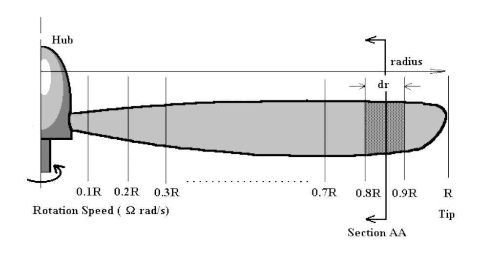
A propeller blade can be subdivided as shown into a discrete number of sections. For each section the flow can be analysed independently if the assumption is made that for each there are only axial and angular velocity components and that the induced flow input from other sections is negligible. Thus at section AA (radius = $r$) shown above, the flow on the blade would consist of the following components.
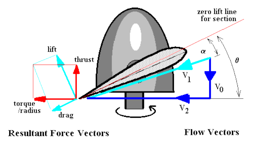
where $V_0$ is the axial flow at propeller disk, $V_2$ is angular flow velocity vector and $V_1$ is section local flow velocity vector, the summation of vectors $V_0$ and $V_2$
Since the propeller blade will be set at a given geometric pitch angle ($θ$) the local velocity vector will create a flow angle of attack on the section. Lift and drag of the section can be calculated using standard 2-D aerofoil properties. (Note: propellers use a changed reference line : zero lift line not section chord line). The lift and drag components normal to and parallel to the propeller disk can be calculated so that the contribution to thrust and torque of the compete propeller from this single element can be found.
The difference in angle between thrust and lift directions is defined as
$$φ=θ-α$$
The elemental thrust and torque of this blade element can thus be written as
$$ΔT=ΔL\cos(φ)-ΔD\sin(φ)$$
$${ΔQ}/r=ΔD\cos(φ)+ΔL\sin(φ)$$
Substituting section data (CL and CD for the given $α$) leads to the following equations.
$$ΔL=C_L 1/2 ρV_1^2 c.dr$$
$$ΔD=C_D 1/2 ρV_1^2c.dr$$
per blade, where $ρ$ is the air density, $c$ is the blade chord so that the lift producing area of the blade element is $c.dr.$
If the number of propeller blades is $B$ then,
$$ΔT=1/2 ρV_1^2c(C_L\cos(φ)-C_D\sin(φ))B.dr\text" (1)"$$
$$ΔQ=1/2 ρ V_1^2c(C_D\cos(φ)+C_L\sin(φ))B.r.dr\text" (2)"$$
Inflow Factors
A major complexity in applying this theory arises when trying to determine the magnitude of the two flow components $V_0$> and $V_2$. $V_0$ is roughly equal to the aircraft's forward velocity ($V_∞$) but is increased by the propeller's own induced axial flow into a slipstream. $V_2$ is roughly equal to the blade section's angular speed ($Ωr$) but is reduced slightly due to the swirling nature of the flow induced by the propeller. To calculate $V_0$ and $V_2$ accurately both axial and angular momentum balances must be applied to predict the induced flow effects on a given blade element. As shown in the following diagram, the induced components can be defined as factors increasing or decreasing the major flow components.
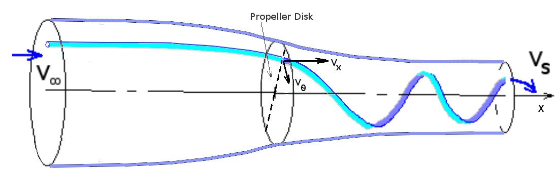
A typical streamtube of flow passing through section AA would have velocities
$$V_{θ}=bΩr\text" and "V_x=V_{∞}(1+a)$$
So for the velocities $V_0$ and $V_2$ as shown in the previous section flow diagram,
$$V_0=V_{∞}+aV_{∞}$$
where $a$ is the axial inflow factor and
$$V_2 = Ωr-bΩr$$
where $b$ is the angular inflow factor (swirl factor)
The local flow velocity and the angle of attack for the blade section is thus
$$V_1=√{V_0^2+V_2^2}\text" (3)"$$
$$α=θ-\tan^{-1}(V_0/V_2)\text" (4)"$$
Axial and Angular Flow Conservation of Momentum
The governing principle of conservation of flow momentum can be applied for both axial and circumferential directions. For the axial direction, the change in flow momentum along a stream-tube starting upstream, passing through the propeller at section AA and then moving off into the slipstream, must equal the thrust produced by this element of the blade.
To remove the unsteady effects due to the propeller's rotation, the stream-tube used is one covering the complete area of the propeller disk swept out by the blade element and all variables are assumed to be time averaged values.
\[ \table ΔT, =, \text "Change in Momemtum flow rate through tube at disk"; , =, \text "Mass flow rate in tube x Change in velocity along tube"; , =, ρ.2πr.dr.V_0×(V_s-V_{∞})\]
By applying Bernoulli's equation and conservation of momentum, for the three separate components of the tube, from freestream to face of disk, from rear of disk to slipstream far downstream and balancing pressure and area versus thrust, it can be shown that the axial velocity at the disk will be the average of the freestream and slipstream velocities.
$$V_0={V_{∞}+V_s}/2$$
which means that
$$V_s=V_{∞}(1+2a)$$
Therefore
\[\table ΔT, =,2πrρV_{∞}(1+a)(V_{∞}(1+2a)-V_{∞}).dr; , =,4πrρV_{∞}^2(1+a)a.dr \text" (5)"\]
For angular momentum
\[\table ΔQ, =,\text"Change in angular momentum rate of flow in tube x radius"; , =,\text"Mass flow rate in tube x change in circumferential velocity x radius"; , =,ρ.2πr.dr.V_0×(V_{θ(slipstream)}-V_{θ(freestream)})×r \]
By considering conservation of angular momentum in conjunction with the axial velocity change, it can be shown that the angular velocity in the slipstream will be twice the value at the propeller disk.
$$V_{θ(slipstream)}=2bΩr\text" and "V_{θ(freestream)}=0$$
Thus
\[\table ΔQ, =, 2πrρV_{∞}(1+a)(2bΩr)r.dr; , =, 4πr^3V_{∞}(1+a)bΩ.dr\text" (6)" \]
Because these final forms of the momentum equation balance still contain the variables for element thrust and torque, they cannot be used directly to solve for inflow factors. However there now exists a nonlinear system of equations (1),(2),(3),(4),(5) and (6) containing the four primary unknown variables $ΔT, ΔQ, a, b$, so an iterative solution to this system is possible.
Iterative Solution procedure for Blade Element Theory.
The method of solution for the blade element flow will be to start with some initial guess of inflow factors $a$ and $b$. Use these to find the flow angle on the blade (equations (3),(4)), then use blade section properties to estimate the element thrust and torque (equations (1),(2)). With these approximate values of thrust and torque equations (5) and (6) can be used to give improved estimates of the inflow factors $a$ and $b$.
This process can be repeated until values for $a$ and $b$ have converged to within a specified tolerance.
It should be noted that convergence for this nonlinear system of equations is not guaranteed. It is usually a simple matter of applying some convergence enhancing techniques (ie Crank-Nicholson under-relaxation) to get a result when linear aerofoil section properties are used. When non-linear properties are used, ie including stall effects, then obtaining convergence will be significantly more difficult.
For the final values of inflow factor $a$ and $b$ an accurate prediction of element thrust and torque will be obtained from equations (1) and (2).
Propeller Thrust and Torque Coefficients and Efficiency.
The overall propeller thrust and torque will be obtained by summing the results of all the radial blade element values.
$$T=ΣΔT \text" (for all elements) and "Q=ΣΔQ \text" (for all elements)"$$
The non-dimensional thrust and torque coefficients can then be calculated along with the advance ratio at which they have been calculated.
$$C_T={T}/{ρn^2D^4}$$
and
$$C_Q={Q}/{ρn^2D^5}$$
where n is the rotation speed of propeller in revs per second and $D$ is the propeller diameter.
The efficiency of the propeller under these flight conditions will then be
$$η_{prop}={JC_T}/{2πC_Q}$$
where advance ratio $J=V_{∞}\/{nD}$.
Software Implementation of Blade Element Theory
Two programming versions of this propeller analysis technique are available. The first is a demonstration program which can be used to calculate thrust and torque coefficients and efficiency for a relatively simple propeller design using standard linearised aerofoil section data. The blade is assumed to have a constant pitch (p) so that the variation of θ with radius is calculated from the standard pitch equation.
$$p=2πr\tan(θ)$$
Click here to run the Propeller Analysis Program Propel
Click here to download the Propeller Analysis Program Propel.exe (MS Windows 32-bit Executable)
Click to download a MATLAB script file for the implementation of this method. The source code in this script is by default a simple propeller design with linear properties. However with the inclusion of your own propeller geometry and section data a more accurate analysis of the specific propeller design can be obtained. Propeller MATLAB script: Propel.m