SUBSONIC COMPRESSIBILITY CORRECTIONS
Potential flow solutions in two and three dimensions give accurate results for aerofoil and wing analysis provided the flow Mach number is less that 0.4. In this low subsonic region the flow is incompressible so that no density variations need to be considered in the governing equations. For higher Mach numbers the density does change, so an extra variable is introduced into the governing equations. The usual conservation of mass equation for two dimensional flow then becomes,
$${∂ρu}/{∂x}+{∂ρv}/{∂y}=0$$
With an extra unknown, an extra governing equation must be invoked to obtain a solution, so the conservation of momentum equation (Euler equ.) is added,
$$u{∂u}/{∂x}+v{∂u}/{∂y}=-1/ρ{∂P}/{∂x}$$
$$u{∂v}/{∂x}+v{∂v}/{∂y}=-1/ρ{∂P}/{∂y}$$
As momentum is a directional quantity, this produces two gradient equations. The flow is still assumed to be inviscid and these equations represent the change of flow momentum in a given direction due to the pressure forces in that direction.
This system of equations can be solved using complex numerical schemes (CFD) but as high speed aerofoil and wing flow is dominated by the stream direction with only small perturbations from this direction, simplifying assumptions can be made to convert the equations to a simple incompressible flow solution method.
The properties of air can be assumed to be a perfect, isentropic gas, $P=ρRT$ (perfect gas law) and with a disturbance speed of $a=√{γRT}$ (speed of sound in air). From the application of these isentropic flow conditions , $P/ρ^γ = \text"constant"$ , the following gas dynamic relation (see section on Gasdynamics - Speed of Sound) can be applied,
$${∂P}/{∂ρ}=a^2$$
The terms of the continuity equation and the pressure gradient components of the Euler equation can be expanded as,
$${∂P}/{∂x}={∂P}/{∂ρ}{∂ρ}/{∂x}=a^2{∂ρ}/{∂x}$$
$${∂P}/{∂y}={∂P}/{∂ρ}{∂ρ}/{∂y}=a^2{∂ρ}/{∂y}$$
$${∂ρu}/{∂x}=u{∂ρ}/{∂x}+ρ{∂u}/{∂x}$$
$${∂ρv}/{∂y}=v{∂ρ}/{∂y}+ρ{∂v}/{∂y}$$
Substituting these terms into the continuity equation,and dividing by density, gives,
$${∂u}/{∂x}-u^2/a^2{∂u}/{∂x}-{uv}/a^2{∂u}/{∂y}+{∂v}/{∂y}-v^2/a^2{∂v}/{∂y}-{uv}/a^2{∂v}/{∂x}=0$$
as the flow is inviscid and hence irrotational,
$${∂v}/{∂x}-{∂u}/{∂y} =0$$
hence continuity simplifies to,
$${∂u}/{∂x}(1-u^2/a^2)-2{uv}/a^2{∂u}/{∂y}+{∂v}/{∂y}(1-v^2/a^2)=0$$
Assuming that the stream velocity, $V_∞$, dominates the flow, then this allows the definition of perturbation velocities, u' and v' such that
$$u=V_∞+u^'\text" and "v=v^'$$
where the prime values represent only small directional disturbances to the stream velocity. Substituting this definition into the continuity equation gives,
$${∂u^'}/{∂x}(1-{(V_∞+u^')^2}/a^2)-2{(V_∞+u^')v^'}/a^2{∂u^'}/{∂y}+{∂v'}/{∂y}(1-{v^{'2}}/a^2)=0$$
If only terms of primary magnitude are kept,
$${∂u^'}/{∂x}(1-V_∞^2/a^2)+{∂v^'}/{∂y} = 0$$
and if the analysis is extended to three dimensions,
$${∂u^'}/{∂x}(1-M_∞^2)+{∂v^'}/{∂y}+{∂w^'}/{∂z}=0$$
This is similar in form to the original governing continuity equation for incompressible flow but with an additional multiplier on the x-direction component. Its solution can be obtained in a similar fashion to the incompressible flow solution procedure.
A perturbation velocity potential $φ^'$ can be defined such that,
$${∂φ^'}/{∂x}=u^'\text" , "{∂φ^'}/{∂y}=v^'\text" , "{∂φ^'}/{∂z}=w^'$$
and on substitution the governing equation becomes,
$$(1-M_∞^2){∂^2φ^'}/{∂x^2}+{∂^2φ^'}/{∂y^2}+{∂^2φ^'}/{∂z^2} =0$$
Without the constant multiplier for the x-direction gradient, this equation would be exactly the same as the potential flow governing equation. A simple solution technique is to apply a geometric scaling transform to the x-direction so that the multiplier is canceled in the second flow field and the solution for the new geometry will be carried out using just potential flow.
The transform scaling multiplier will be $β=1-M_∞^2$. This will be applied to x-dirn only. The transformed geometry will be $x^'=x/β\text", "y^'=y\text" and "z^'=z$. This will lead to a new geometry with the same thickness and span but a longer chord as the scaling factor is always less than 1.
Substituting into the governing compressible flow equation gives,
$$β^2{∂^2φ^'}/{∂(βx^')^2}+{∂^2φ^'}/{∂y^{'2}}+{∂^2φ^'}/{∂z^{2^'}} =0$$
$${∂^2φ^'}/{∂x^{'2}}+{∂^2φ^'}/{∂y^{'2}}+{∂^2φ^'}/{∂z^{'2}} =0$$
This standard Laplace equation in perturbation potential for the transformed flow field can be solved using the usual potential flow techniques for aerofoil sections and wings as shown previously in this chapter.
Note that for two dimensional, section solutions, the transformed geometry is just a smaller thickness to chord ratio version of the original geometry. In most cases this can be assumed to have the same incompressible “thin aerofoil” solutions as the original geometry. For three dimensional wings, the new geometry has a reduced aspect ratio so these solutions will need to be predicted separately for this geometry.
In all cases, inviscid, incompressible flow solutions for velocities $u^'$, $v^'$, $w^'$ and then pressures and forces $Cp^'$, $C_L^'$ ...etc, can be easily found. These then need to be transformed back (inverse transform) to find their equivalent values for the original compressible flow field. For velocity,
$$u^'(x,y,z)={∂φ^'}/{∂x}$$
$$u^'(x^',y^',z^')={∂φ^'}/{∂x^'}={∂φ^'}/{∂βx}$$
thus the horizontal perturbation velocity in the original flow field is scaled by the factor β compared to the component in the incompressible flow field. The other component velocities are unchanged.
$$u^'(x,y,z)=1/βu^'(x^',y^',z^')$$
To determine the pressure scaling, a compressible version of the Bernoulli equation (based on conservation of momentum) can be applied along a stream tube flowing over the aerofoil.
$$V_∞^2/2-V^2/2=∫_{P_∞}^{P}1/ρ.dP$$
Assuming small perturbation properties,
$$V^2=(V_∞+u^')^2+v^{'2}+w^{'2}≈V_∞^2+2V_∞u^'$$
and
$$ρ=ρ_∞+ρ^'≈ρ_∞$$
Substituting and expanding the integration gives,
$$V_∞^2/2-(V_∞^2/2-{2V_∞u^'}/2)={P-P_∞}/ρ_∞$$
Hence the pressure coefficient for the compressible flow will be,
$$Cp={P-P_∞}/{1/2ρ_∞V_∞^2}=-{2u^'}/V_∞$$
Comparing this between the two parts of the transformed flow gives the mapping of pressure coefficient between the two.
$$Cp=-{2u^'(x,y,z)}/V_∞=-1/β {2u^'(x^',y^',z^')}/V_∞={Cp^'}/β$$
The compressible flow field coefficients can be found by scaling the incompressible flow field coefficients by the factor, $1/β=1/√{1-M_∞^2}$ .
The force coefficients will scale in the same manner as the pressure coefficients. Although the lengths are different between the two flow fields, the non-dimensionalising of the length scales will correct for this. In fact, this potential flow result could be generalised to all force coefficients for a subsonic compressible flow, if the incompressible results are known.
$$C_L={C_L(\text"incompressible")}/√{1-M_∞^2}$$
$$C_D={C_D(\text"incompressible")}/√{1-M_∞^2}$$
$$C_M={C_M(\text"incompressible")}/√{1-M_∞^2}$$
Limiting Case, Critical Mach Number.
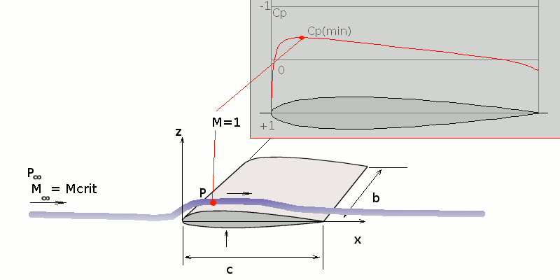
This simple compressible flow correction theory works reasonably well up to the point where supersonic flow starts to appear near the surface of the aerofoil section. This will happen before the free-stream becomes supersonic due to the acceleration of the air in the vicinity of the aerofoil. Supersonic flow obeys different physical rules as the flow is moving faster than disturbances can propagate within the gas, (speed of sound) and the assumptions of a simple perturbation theory are no longer are valid. The free-stream Mach number for which supersonic flow first occurs on the wing or section is called the critical Mach number. Not only is this an important limit for theory but also marks the start of transonic flow and the likely-hood of a significant drag rise for the section.
In order to predict the critical Mach number, the above compressibility correction factor can be combined with standard gas dynamic equations. This is not a linear first order problem so analysis may be a bit difficult.
Sample pressure fields for NACA 0012 aerofoil section at 0 deg angle of incidence and a range of subsonic and transonic Mach numbers are shown in the following figure. High pressure is shown as red, low pressure as blue.
Critical Mach number is approx 0.7 for this case. A significant difference in flow structure can be observed between high subsonic flow (0→0.65) and transonic flow (0.75→1.5).
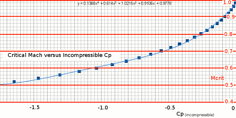
Critical Mach number will vary for aerofoils and wings depending on their angle and camber as this determines the minimum pressure coefficient point, the point at which the local flow is fastest. This will be the point at which the flow first becomes supersonic, $M=1$.
Minimum pressure coefficient for incompressible flow, $Cp^'$ can be found using potential flow techniques. By applying the subsonic correction factor, minimum pressure coefficient for compressible flow can be found,
$$Cp(min)={Cp^'(min)}/√{1-M_∞^2}$$
However as speed where $M_∞=M_{crit}$ is still unknown, this leads to a complex second order problem.
The variation of pressure along the stream tube can be used to provide another estimate of $Cp$. The following is the full gas dynamics equation solution (see Compressible Flow Section – Isentropic Relations.)
$$P/P_∞=({1+{γ-1}/2 M_∞^2}/{1+{γ-1}/2 M^2})^{γ/{γ-1}}$$
Search for the point where $P=P(min)$ at $M=1$, then this corresponds to the condition when free-stream Mach number is $M_{crit}$,
$$P_{min}/P_∞=({1+{γ-1}/2 M_{crit}^2}/{1+{γ-1}/2})^{γ/{γ-1}}$$
Thus a second expression for $C_P(min)$ is,
$$Cp(min)={P_{min}-P_∞}/{1/2 ρ_∞V_∞^2}={P_{min}-P_∞}/{1/2γP_∞M_{crit}^2}$$
$$Cp(min)=2/{γM_{crit}^2}(P_{min}/P_∞-1)$$
Substituting the compressibility correction factor and the above expression for pressure ratio, leads to the following equation.
$${Cp^'(min)}/√{1-M_{crit}^2}=2/{γM_{crit}^2}(({2+(γ-1)M_{crit}^2}/{γ+1})^{γ/{γ-1}}-1)$$
Given a value of the incompressible flow minimum pressure coefficient for a wing or section at set free-stream flow angle, it should theoretically be possible to solve for the critical Mach number of the section at that condition. However as the equation is highly non-linear and difficult to invert, the solution is obtained either by an iterative process or by plotting minimum pressure coefficient versus critical Mach number and using empirical data lookup or curve fitting.
The following is a plot of minimum incompressible pressure coefficient versus critical Mach number.