2D PANEL METHODS
The prediction of aerodynamic properties of streamlined aerofoil sections can be obtained relatively quickly and accurately using two dimensional panel method analysis. The solutions will be initially inviscid flow predictions. This will give lift and pitching moment properties. Then, with the introduction of some simple one-dimensional boundary layer theory, the viscous component of the solution can be predicted and drag calculated.
The solution is obtained by combining two separate calculations, an inviscid panel method prediction of flow velocities and pressures and a viscous boundary layer theory prediction of surface flow displacement and momentum loss due to friction.
Because the presence of a boundary layer does modify the aerofoil's displacement effect on the freestream, it is more accurate to iterate between the results of these two solutions and obtain a final, converged solution. However in many cases, numerical problems may arise due to the number of iterations required and the possibility of an unstable iteration.
In the Reynolds number range that is the case for small to large aircraft, the boundary layer is very thin and a reasonable result is generally obtained by just using a single pass of each solution component. The solution software below does just one inviscid flow solution for velocities and then one boundary layer integration pass to obtain a solution. More complex panel method solutions are available in the reference material listed below.
Inviscid Panel Method
A potential flow solution of any general aerofoil section can be modeled by discretising the surface contour using singularity panels. Many different techniques are possible but for the programs used on this site, the following configuration has been employed for the panel modeling. It is based on using straight panels with a linear distribution of vorticity between end points.
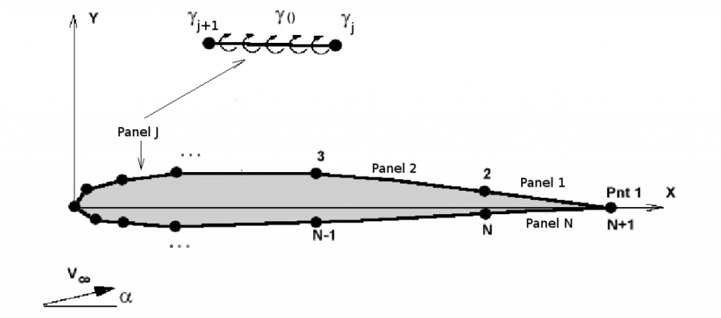
Each panel is a straight line segment between surface contour points $j$ and $j+1$. Along the panel, a vortex distribution of linearly varying strength $γ$ is applied with a pair of constant values at each end point, $γ_j$ and $γ_{j+1}$. This distribution strength varies from panel to panel but end point values must be consistent. As the geometry of the section and the freestream flow conditions $V_∞$ -- velocity , $α$ -- angle of attack ) are set, the requirement will be to define boundary condition equations in order to determine the necessary distribution strength at the panel end points $γ_j, j=1,N$ where $N$ is the number of panels) for an accurate model of the problem.
A boundary condition of no flow through surface $V_n=0$ can be applied at the center of each panel. This produces $N$ equations in $N+1$ unknowns. In order to correctly solve for the extra unknown vorticity, a Kutta condition must be applied at the trailing edge.
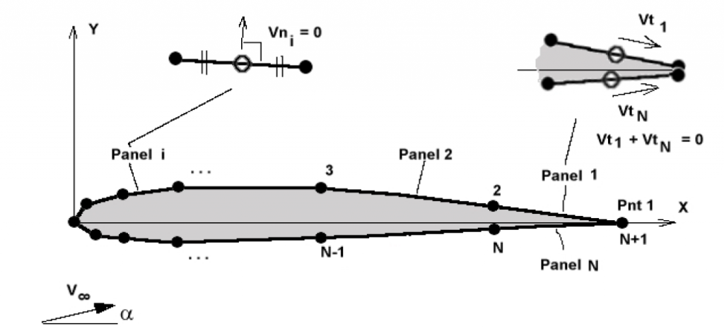
For a single panel $i$ the boundary condition will be applied as,
$$V_n = Σ ( \text"velocities on panel due to all panel vorticies" ϒ ) + \text"freestream velocity component" = 0$$
$$V_n=∑_{j=1}^{N+1}(A_{i,j}.γ_j)+B_iV_∞=0\text" at Panel (i)"$$
where the coefficient, $A_{i,j}$,represents the influence of the vorticity components of panel $j$ on the control point on panel $i$ and , $B_i$, represents the influence of the freestream on panel $i$. All coefficients are functions of the geometry of the section, Ai,j = function(x,y) due to orientation and spacing of panels.
The Kutta condition, equation $N+1$ can be applied in terms of trailing edge tangential velocities which means that the vorticity at the trailing edge is zero,
$$V_{t.e.}(\text"upper surface")=-V_{t.e.}(\text"lower surface")\text" , "V_{t.e.}(1)=-V_{t.e.}(N)\text" , "γ_{t.e.}=0$$
thus
$$γ_1+γ_{N+1}=0$$
This gives a system of linear equations which allow the solution for the required distribution strengths to be found.
$$ [ {\table A_{1,1}, A_{1,2}, ..., A_{1,N+1}; A_{2,1}, A_{2,2}, ..., A_{2,N+1}; , ... , , ; A_{N,1}, A_{N,2}, ..., A_{N,N+1}; 1, 0 , ..., 1} ] × ( {\table γ_1; γ_2; .; γ_N; γ_{N+1} } ) = - ( {\table B_1; B_2; .; B_N; 0 } ) V_∞ $$
Once the distribution strengths $γ_j$ have been calculated, surface tangential velocities at the centre of each panel can be calculated $V_i$ and then surface pressure coefficients $Cp_i$,
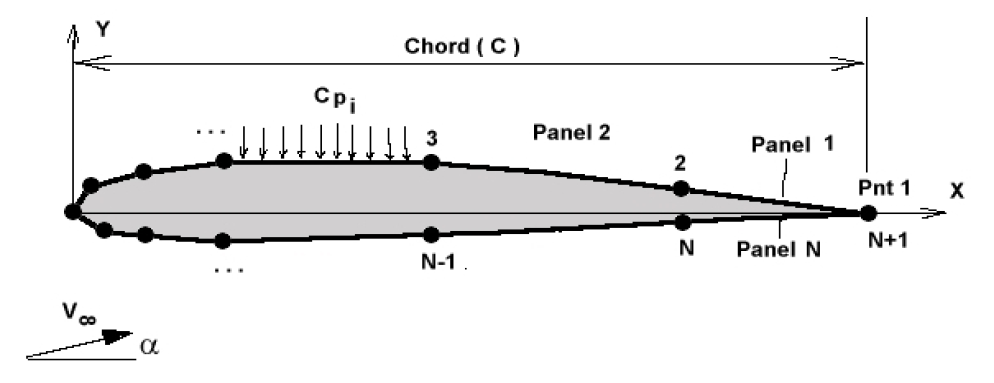
$$Cp_i=(1 - V_i^2/V_∞^2)$$
The lift coefficient can be calculated, assuming a small angle of attack, as the integration of surface pressure coefficient acting in the y-direction, ie. projected on the x axis.
$$C_L = ∑_{i=1}^N Cp_i {(x_i-x_{i+1})}/c$$
Pitching moment coefficient will similarly be the sum of the panel moments about the 1/4 chord point.
$$C_{M 1/4 c}= ∑_{i=1}^N Cp_i {(x_i-x_{i+1})}/c ({(x_i+x_{i+1})}/{2c} - 1/4)$$
Both calculations assume the cos(α) effect due to the difference between chord line and freestream direction are negligible.
Solutions only need to be calculated for one or two angles of attack as the lift curve will be linear. Stall and boundary layer effects are not predicted by the first part of the process as it deals only with inviscid flow.
APPLICATION : 2D Panel Code Computer Program.
The following program accepts ASCII data files which consist of a list 2-D aerofoil section coordinate points (x,y). The format of these aerofoil input data files is the same as that produced by the NACA section generation program.
The data file structure used is shown below,
Header Line
N (Number of Data Points describing section)
X(1) Y(1)
X(2) Y(2)
X(3) Y(3)
...
X(N) Y(N)
There is an initial header line, followed by a line giving the number of data points used to describe the aerofoil and then pairs of surface coordinate points (x,y). The order of surface points is anti-clockwise, starting at the trailing edge, going back over the upper surface around the nose and then forward along the underside back to the trailing edge. Data files for other aerofoil sections can be created using a spreadsheet or text editor to give a data file in the correct format.
Some sample section files are NACA 0012, NACA 4412 and NACA 64-012.
From the surface coordinate data file, the program calculates an inviscid flow solution. The 1-D momentum integration is run to predict the boundary layer near the aerofoil surface. The program can predict CL, Cm(1/4c) and CD for the specified aerofoil section at a given angle and Reynolds number.
- Executable Program : 2-D Panel Method Solution MS Windows downloadable
- Executable Program : 2-D NACA Aerofoil Section Generator MS Windows downloadable
- Virtual Wind Tunnel System : Program Suite to allow a number of different solutions
- Alternately for a more elaborate section solver try the XFOIL program, visit the Marc Drela GPL Aerofoil Solution System site at MIT XFOIL site.