3D PRANDTL LIFTING LINE THEORY
Application to high aspect ratio, unswept wings.
A simple solution for unswept three-dimensional wings can be obtained by using Prandtl's lifting line model. For incompressible, inviscid flow, the wing is modelled as a single bound vortex line located at the 1/4 chord position and an associated shed vortex sheet.
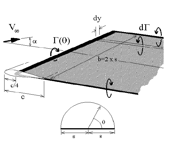
where $Γ$ is the circulation (vortex strength), defined a function across the wing span, $V_∞$ is free-stream velocity, $b$ is wing span, $s$ is wing semi-span, $c$ is wing chord and $y$ is the distance across the span measured from the wing root. The mapping of angle $θ$ to semi-span $s$ position is done using Fourier series and allows variation of the model to suit different geometries.
$$y=s\cos(θ)$$
The span-wise lift distribution is assumed to be approximately elliptical with a small modifications due to wing plan-form geometry. The vortex line strength can thus be modelled using the following Fourier series approximation,
$$Γ(y)=Γ(θ)=4sV_∞ ∑_{n=1}^{∞} A_n \sin(nθ)$$
The required strength of the distribution coefficients $A_n$ for a given geometry and set of free-stream conditions can be calculated by applying a surface flow boundary condition. The equation used is based on the usual condition of zero flow normal to the surface.
$$V_n=0$$
For 3-D wings this condition is applied at several span-wise locations. By matching flow and surface angles, the normal velocity boundary condition can be restated as a requirement for the flow angles at the section to be in balance. Unlike 2-D section flow where flow angles are set by freestream direction and surface angles only, in 3-D wing flow an extra flow angle component is introduced by the shed vortices that are produced and trail behind the wing. This trailing vortex sheet produces a downwash. For a 3-D wing, the local section flow angle must be equal to the sum of the wing's angle of attack, the section twist and the downwash induced flow angle.
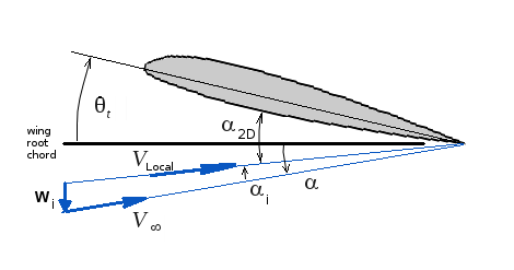
$$α_{2D}=α-α_i+θ_t$$
where
$$α_i=w_i/V_∞$$
and where $α$ is the 3-D wing angle of attack, $θ_t$ is the wing twist angle and $w_i$ is the velocity induced by trailing vortex sheet. The downwash velocity is caused by the shed vorticies trailing behind the wing. The vortex strength in the trailing sheet will be a function of the changes in vortex strength along the wing span. The mathematical function describing the vortex sheet strength is thus obtained by differentiating the bound vortex distribution.
$$dΓ=4sV_∞∑_{n=1}^{∞}nA_n\cos(nθ).dθ$$
Thus the downwash at any span position on the wing can be found by integrating the influence of individual elements of the trailing sheet. Each sheet element behaves like 1/2 of an infinite vortex line so
$$dw_i=Γ/{4πr}$$
where $r$ is the distance across the span between the vortex element and the point at which downwash is being calculated. $r=(y–y_i)$. The full downwash will be,
$$w_i=1/{4π}∫_{-s}^{+s} 1/{y-y_i} .dΓ$$
On substitution of the mapping variables and integration, the result is,
$$w_i={V_∞}/{π}∫_{0}^{π} 1/{\cos(θ_i)-\cos(θ)} ∑_{n=1}^{∞}nA_n\cos(nθ).dθ$$
$$w_i=V_∞∑_{n=1}^{∞}{nA_n\sin(nθ_i)}/{\sin(θ_i)}$$
The 2-D section lift coefficient is a function of the local flow incidence and the bound vortex strength at this span location. So that,
$$C_{L_{2D}}=a_0(α_{2D}-α_0)=Γ/{V_∞c}$$
where $a_0$ is the section lift slope $dC_L\/dα_{2D}, α_0$ is the section zero lift angle and $c$ is the chord length. This can be rearranged in terms of vortex strength,
$$Γ=1/2 a_0V_∞c(α-α_i+θ_t-α_0)_$$
and substituting for vortex strength and induced angle produces the following boundary condition equation at a point $θ=θ_i$,
$$4sV_∞∑_{n=1}^{∞}A_n\sin(nθ)=1/2 a_0 V_∞c(α- ∑_{n=1}^{∞}{nA_n\sin(nθ)}/{\sin(θ)}+θ_t-α_0)$$
$$∑_{n=1}^{∞}A_n\sin(nθ)(\sin(θ)+n {a_0c}/{8s})={a_0c}/{8s}\sin(θ)(α+θ_t-α_0)$$
where the term ${a_0c}/{8s}$ is usually simplified as $μ$.
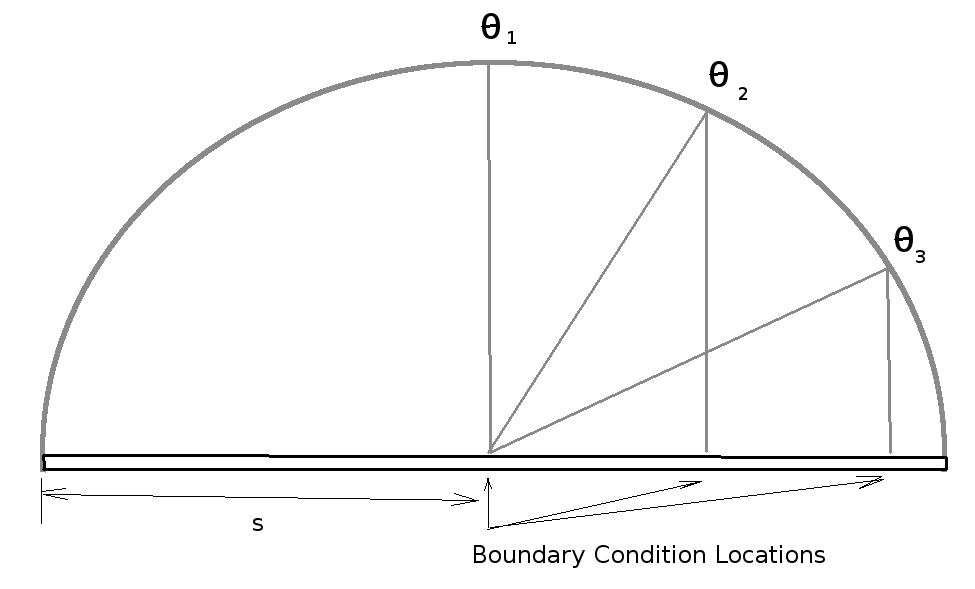
This final boundary equation contains all the unknown coefficients of the wing model's vortex distribution, along with the wing's geometry and the stream conditions. It can be used to find coefficients $A_1,A_2,A_3,$ ... Assuming that higher order coefficients become increasingly small and make negligible contribution to the result, one method of solution is to truncate the series at term $A_N$. By applying the boundary condition at $N$ span locations ($θ_i,i=1,N$) a set of simultaneous linear equations can be constructed. This set can be solved for coefficients $A_1$ to $A_N$. A cosine distribution of span-wise locations should be used for the boundary conditions to match the assumed wing loading distribution. Clearly the number of coefficients used will determine the accuracy of the solution. If the wing loading is highly non-elliptical then a larger number of coefficients should be included. This occurs when analysing wings with part span flaps. This type of geometry causes a discontinuity in the spanwise loading and hence requires a much larger number of coefficients to accurately describe the distribution. Where the the wing loading is symmetric about the wing root, the contribution of even functions will become zero. Coefficients $A_2,A_4,A_6,$ ... are all zero and can be dropped from the analysis.
For example, for an untwisted wing with constant chord $c$ and constant aerofoil section $a_0, α_0$ across the span, setting $N=5$ for a symmetric loading with $A_2=A_4=0$, would require evaluation of the boundary condition at 3 locations $θ=π/2, π/3$ and $π/6$
which produces the following matrix,
$$ [ {\table \sin(θ_1)(\sin(θ_1)+μ), \sin(3θ_1)(\sin(θ_1)+3μ), \sin(5θ_1)(\sin(θ_1)+5μ) ; \sin(θ_2)(\sin(θ_2)+μ), \sin(3θ_2)(\sin(θ_2)+3μ), \sin(5θ_2)(\sin(θ_2)+5μ); \sin(θ_3)(\sin(θ_3)+μ), \sin(3θ_3)(\sin(θ_3)+3μ), \sin(5θ_3)(\sin(θ_3)+5μ) } ] × ( {\table A_1;A_3;A_5}) = ({\table μ\sin(θ_1)(α-α_0); μ\sin(θ_2)(α-α_0); μ\sin(θ_3)(α-α_0);} )$$
For a given angle of attack $α$, the system can be solved for $A_1,A_3$ and $A_5$ to give the wing load distribution.
Once the coefficients of the load distribution are known the total lift of the wing can be found by integration.
$$\text"Lift"=ρV_∞∫_{-s}^{+s}Γ.dy = ρV_∞∫_{0}^{π}4sV_∞∑_{n=1}^{∞}A_n\sin(nθ).s\sin(θ).dθ$$
as only $\sin^2(θ)$ integration is non zero this gives,
$$L=ρs^2V_∞^2 . 2πA_1$$
which reduces to a lift coefficient of
$$C_L = π.AR.A_1$$
where $AR$ is the aspect ratio of the wing
$$AR = b^2/S = {4s^2}/S$$
A consequence of the downwash flow is that the direction of action of each section's lift vector is rotated relative to the free-stream direction. The local lift vectors are rotated backward and hence give rise to a lift induced drag. While the overall governing equations are potential flow and hence do not give rise to friction or pressure drag, this lift induced drag will be a significant component of the overall drag of the wing. The downwash velocity induced at any span location can be calculated once the strength of the wing loading is known. The variation in local flow angles can then be found. By integrating the component of section lift coefficient that acts parallel to the free-stream across the span, the induced drag coefficient can be found.
$$D_i=ρV_∞∫_{-s}^{+s}Γ\sin(α_i).dy$$
if small angle approximations are used, $\sin(α_i)=w_i\/V_∞$ which produces the following induced drag coefficient ,
$$C_{Di}=π.AR.∑_{n=1}^{∞}nA_n^2$$
No information about pitching moment coefficient can be deduced from lifting line theory since the lift distribution is collapsed to a single line along the 1/4 chord. All forces will be centered at the 1/4 chord in this model irrespective of aerofoil section geometry.
Special Case of Purely Elliptical Wing Loading
If the wing planform is elliptical, $c=c_0\cos(θ)$ then it can be shown that the wing load distribution is also a purely elliptical function and all coefficients except $A_1$ will vanish.
$$Γ(y)=Γ(θ)=Γ\sin(θ)=4sV_∞\sin(θ)$$
For simple straight and tappered, unswept and untwisted wings, this solution may be used as a first approximation. For these geometries all other coefficients will be much less than $A_1$ and the loading will be approximately elliptical. In this case, a single general boundary condition equation results containing only one unknown, the vortex line strength at the wing root.
$$Γ_0=4sV_∞A_1$$
The solution of the boundary condition in this case leads to a constant downwash across the span and the following simple answers for lift coefficient and induced drag coefficient.
$${∂C_L}/{∂α}= a_0/{(1+a_0/{πAR})}$$$$α_0(2D)=α_0(3D)$$
$$C_{Di}=C_L^2/{πAR}$$
Reference
Houghton & Carruthers "Aerodynamics for Engineering Students", Arnold Ed 3 1982.
Software : Prandtl Lifting Line Program
The following computer program allows the user to define wing plan-forms (without sweep) and to define wing root and wing tip section properties. The program assumes a linear variation of section properties between wing root and tip. For the MS Windows downloadable version, and that the wing loading is assumed to be symmetric about the wing root.
Section lift data in terms of $a_0, α_0$, ie. $C_L(2D) = a_0(α_{2D} - α_0)$ are required for the wing root and the wing tip sections. This information can be obtained from published 2-D experimental data or theoretical techniques such as thin aerofoil theory.
The program uses the above lifting line equations to get solutions for lift coefficient versus angle of attack and induced drag coefficient versus lift coefficient2. For a given angle of attack the program will display the resulting distribution of section lift coefficient across the span, the distribution of downwash at the wing and a listing of the solution Fourier coefficients for this angle.
A flapped section can also be input. The percentage of wing span with flap must be input to create a flapped wing section. The flap section properties are assumed to be those entered for the wing root section. These section properties will be kept constant across the flapped portion of the span. The section properties used outboard of the flap will also be constant and assumed to be equal to those of the wing tip.
Software
- Prandtl Lifting Line Solver for 3D unswept wings (MS Windows downloadable)