Flight Mechanics* General Equations * Linearised Equations * Longitudinal Motion * Lateral Motion * Aerodynamic Derivatives |
General Equations of Aircraft MotionThese pages are intended to give a substantial grounding in aircraft flight statics and dynamics. To start, an overview of the axis systems used is given to define aircraft motion. The general non-linear equations of aircraft motion arise from the inter-relation of these axis systems and are developed from the general equations of linear and angular motion. In many cases it is more convenient to use a linearised version of the aircraft equations of motion and these will be developed from the general equations. The forces and moments that act on the aircraft determine its motion. These are inputs to the equations but are dependent on the solution variables of the equations (state variables). However using the concept of small amplitude disturbances from a trimed flight condition, a simpler set of equations is obtained that can yield the natural modes of motion and identify dynamic stability. Axis SystemsThe following axis systems are used to define aircraft orientation and motion.
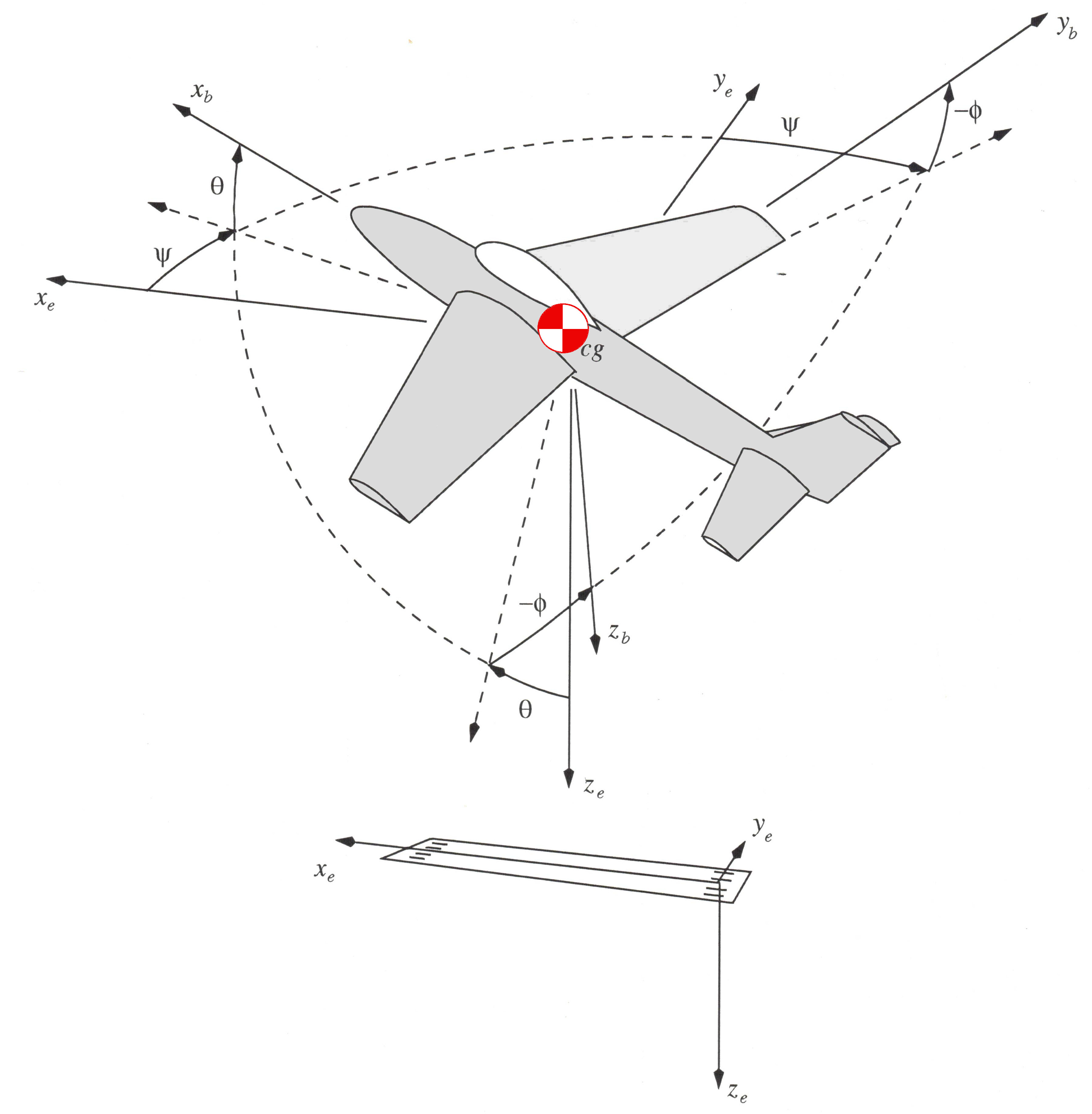
Figure 1: Earth and Body Axes Relationship. 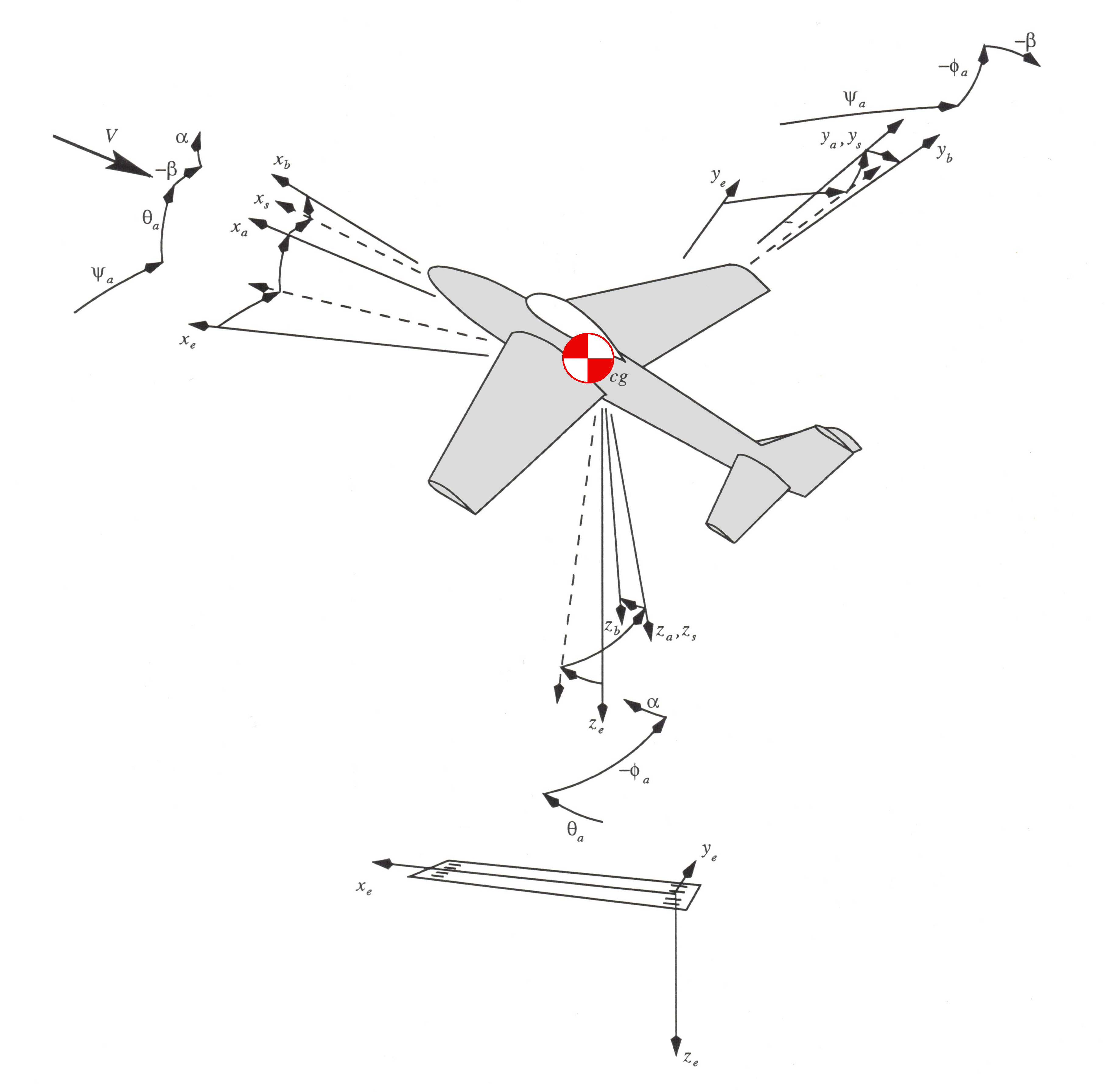 Figure 2 : Earth, Body and Wind Axes Relationship. The motion of a aircraft will be considered with reference to a body centered axis system and an earth fixed axis system which will be considered to be an inertial reference frame for aircraft velocities and path trajectories. (Figure 1.) The aircraft can be considered to be built up of small component elements (Figure 3.). An element of the aircraft will have mass, $dm$, aerodynamic load bearing surface, $dS$, volume, $dV$, and density, $dρ_a$. The aerodynamic and inertial forces will act on it as shown in Figure 3. 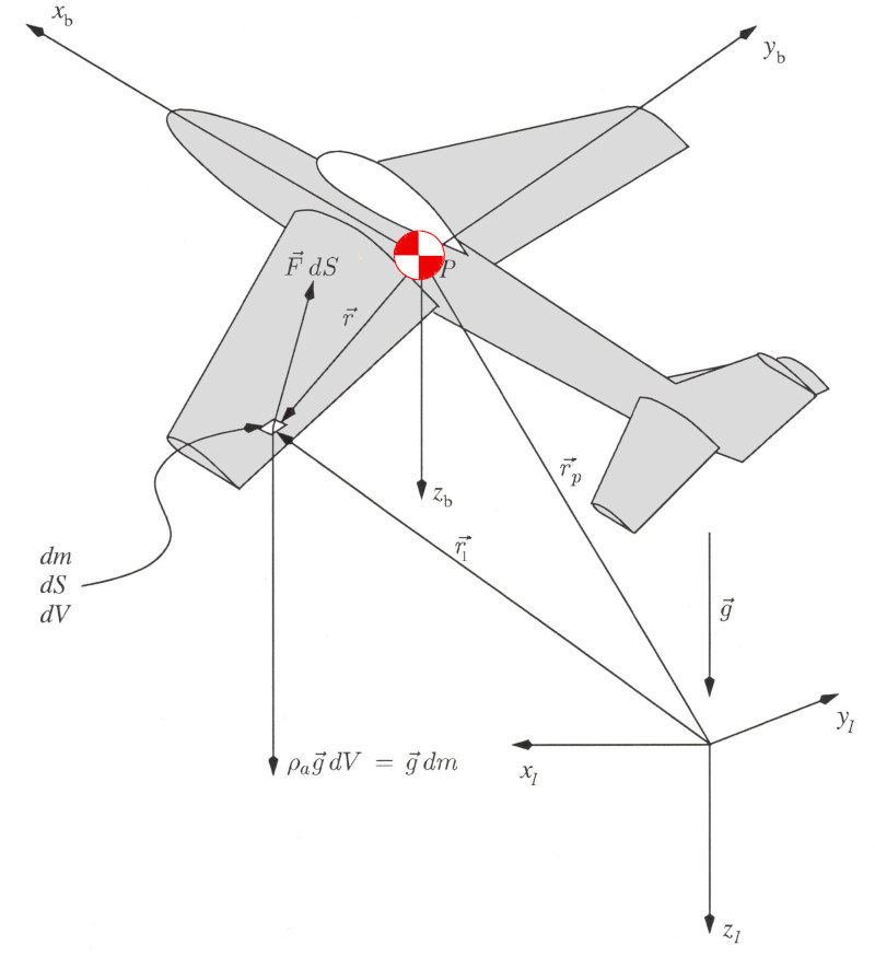
Figure 3. Motion of an aircraft element. Newton’s Law of linear motion and Euler’s Law of angular motion apply in the inertial reference frame and may be applied to the aircraft by integrating over all its component elements. Linear motion gives,
$$d/{dt}[∫_V ρ_a {dr↖{→}_1}/{dt}.dV] =
∫_V ρ_a g↖{→}.dV + ∫_S F↖{→}.dS\text" (1)"$$ Angular motion gives,
$$d/{dt}[∫_V r↖{→}_1 × ρ_a
{dr↖{→}_1}/{dt}.dV] = ∫_V r↖{→}_1
× ρ_a g↖{→}.dV + ∫_S r↖{→}_1 × F↖{→}.dS\text" (2)"$$ Note that these equations are relative to an inertial reference frame ($x_1,y_1,z_1$). In the case of aircraft a simple earth axis (Figure 1) is typically used but in other cases, for example, an orbiting satellite, other inertial systems may be used such as earth centred inertial frame or sun centred reference frame. Translation Only.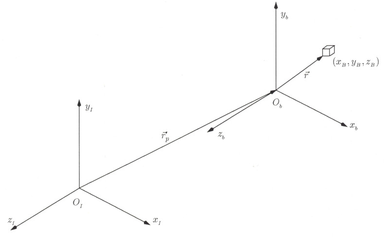
Figure 4. Translation of body axis system relative to inertial system. If an element is subjected to translation motion only, (Figure 4), its position can be described with respect to the inertial frame according to, $$x↖{→}_1=x↖{→}_{1Ob} + x↖{→}_b$$ or $$x↖{→}_1=r↖{→}_{p} + r↖{→}\text" (3)"$$ where $x↖{→}_{1Ob}$ is the location of the body axis origin relative to the inertial frame and $x↖{→}_b$ is the location of the element with respect to the body axes.
Rotation Only.If an element is subjected to rotational motion about the body axes, Figure 5, where $p,q$ and $r$ are the components of the total rotation vector $ω↖{→}$ about the $x_b,y_b$ and $z_b$ axes, $ω↖{→}=pi↖{→}+qj↖{→}+rk↖{→}$, then the position of the element is a function of the rotation vector and the position vector $r↖{→}$ with respect to the body axes.  Figure 5. Rotation of body axes relative to inertial system General Case for MotionIn the general case of a vector in a rotating reference frame, the observed rate of change of any vector depends on the reference frame in which the observer is stationed. If the rotation rate of the ($x_b,y_b,z_b$) axes with respect to ($x_1,y_1,z_1$) is denoted by $ω↖{→}$, then the rate of change of any vector $A↖{→}$ observed from the inertial frame is, $${dA↖{→}}/{dt}= {∂A↖{→}}/{∂t}+ω↖{→} × A↖{→}\text" (4)"$$ where ${∂A↖{→}}/{∂t}$ is the rate of change of $A↖{→}$ viewed from the ($x_b,y_b,z_b$) frame. Linear MotionConsider the linear motion of an aircraft, making the assumption that the body force, gravity, is constant over the body and that surface forces arise from thrust and aerodynamic loads. Then with reference to Fig. 3, $$d/{dt}[∫_V ρ_a d/{dt}({r↖{→}}_p + r↖{→}).dV]=∫_V ρ_a g↖{→}.dV + ∫_S F↖{→}.dS\text" (5)"$$ or $$d/{dt}[∫_V ρ_a d/{dt}({r↖{→}}_p + r↖{→}).dV]= mg↖{→}+{F↖{→}}_A+{F↖{→}}_T\text" (6)"$$ Assuming that the aircraft is a rigid body, so ${dr↖{→}}/{dt}=0$. The aircraft velocity will be the velocity of its centre of mass and in the inertial reference frame this will be $${V↖{→}}_p={d{r↖{→}}_p}/{dt}$$ Also ${V↖{⋅}}_p = {∂V↖{→}}/{∂t}$ is the rate of change of velocity as viewed from the vehicle. Thus, substituting these aircraft assumptions into the equation for the general case of motion and summing over the complete mass, $∫.dm$ of the vehicle, gives from Equ. 4, $$ d/{dt}[∫_V {V↖{→}}_p.dm] = ∫_V ({V↖{⋅}}_p + ω↖{→} × {V↖{→}}_p).dm\text" (7)"$$ So the equation for linear motion, Equ.6, becomes, $$ m[{V↖{.}}_p+ω↖{→} × {V↖{→}}_p]=mg↖{→} + {F↖{→}}_A +{F↖{→}}_T\text" (8)"$$ with variables now referenced to the body centered axes. Angular motionThe left hand side of the general angular motion equation, Equ.2, gives, $$\cl"ma-join-align"{\table d/{dt}[∫_V {r↖{→}}_1 × ρ_a {d{r↖{→}}_1}/{dt}.dV], {= d/{dt}[∫_V ({r↖{→}}_p+r↖{→}) × d/{dt}({r↖{→}}_p +r↖{→}).dm]}; , {= d/{dt}[∫_V {r↖{→}}_p × {d{r↖{→}}_p}/{dt}.dm + ∫_V{r↖{→}}_p × {dr↖{→}}/{dt}.dm + ∫_V r↖{→} × {d{r↖{→}}_p}/{dt}.dm+∫_V r↖{→} × {dr↖{→}}/{dt}.dm]}; , {= d/{dt}[∫_V {r↖{→}}_p × {d{r↖{→}}_p}/{dt}.dm + {r↖{→}}_p × d/{dt}∫_V r↖{→}.dm - {d{r↖{→}}_p}/{dt} × ∫_V r↖{→}.dm + ∫_V r↖{→} × {dr↖{→}}/{dt}.dm]}; , {= d/{dt}[∫_V {r↖{→}}_p × {d{r↖{→}}_p}/{dt}.dm + ∫_V r↖{→} × {dr↖{→}}/{dt}.dm]}}\text" (9)"$$ In the above equation, subscript $p$ denotes quantities relative to the centre of mass $P$ of the aircraft, so $∫_V r↖{→}.dm=0$. The mass is assumed invariant so the time derivatives may be brought outside the integrals. Equ. 9 LHS can be manipulated as follows, $$\cl"ma-join-align"{\table LHS, {= ∫_V[{d{r↖{→}}_p}/{dt} × {d{r↖{→}}_p}/{dt}].dm + ∫_V {r↖{→}}_p × {d^2({r↖{→}}_p)}/{dt^2}.dm+d/{dt}[∫_V r↖{→} × {dr↖{→}}/{dt}.dm]}; , {= {r↖{→}}_p × {d^2}/{dt^2}[ ∫_V {r↖{→}}_p .dm] + d/{dt}[∫_V r↖{→} × {dr↖{→}}/{dt}.dm]}\text" (10)"$$ From the linear momentum equation, $$d/{dt}∫_V {d{r↖{→}}_1}/{dt} .dm - ∫_V g↖{→}.dm - ∫_S F↖{→}.dS=0\text" (11)"$$ so that
$$ {r↖{→}}_p × [d/{dt}(∫_V {d{r↖{→}}_1}/{dt}.dm) - ∫_V g↖{→}.dm - ∫_S F↖{→}.dS] = 0$$ Since then $$ {r↖{→}}_p × d^2/{dt^2}(∫_V {r↖{→}}_p.dm) = {r↖{→}}_p × ∫_V g↖{→}.dm + {r↖{→}}_p × ∫_S F↖{→}.dS\text" (12)"$$ This result can be applied to Equ. 10 to yield, $$ LHS = {r↖{→}}_p × ∫_V g↖{→}.dm + {r↖{→}}_p × ∫_S F↖{→}.dS + d/{dt}[∫_V r↖{→} × {dr↖{→}}/{dt}.dm]\text" (13)"$$(13) Next consider the right hand side of Equ. 2, $$\cl"ma-join-align"{\table ∫_V {r↖{→}}_1 × g↖{→}.dm + ∫_S {r↖{→}}_1 × F↖{→}.dS, {= ∫_V ({r↖{→}}_p+r↖{→}) × g↖{→}.dm + ∫_S ({r↖{→}}_p+r↖{→}) × F↖{→}.dS}; , {= {r↖{→}}_p × ∫_V g↖{→}.dm + ∫_V r↖{→} × g↖{→}.dm + {r↖{→}}_p × ∫_S F↖{→}.dS + ∫_S r↖{→} × F↖{→}.dS}}\text" (14)"$$ If $g$ remains constant over the aircraft, then, $$ ∫_V r↖{→} × g↖{→}.dm = -g↖{→} × ∫_V r↖{→}.dm =0\text" (15)"$$ so that, $$ RHS = {r↖{→}}_p × ∫_V g↖{→}.dm +{r↖{→}}_p × ∫_S F↖{→}.dS + ∫_S r↖{→} × F↖{→}.dS\text" (16)"$$ Equating LHS=RHS (Equ. 13 = Equ. 16) gives the angular momentum equation in the body axis system coordinates but viewed from the inertial frame as, $$ d/{dt}[∫_V r↖{→} × {dr↖{→}}/{dt}.dm] = ∫_S r↖{→} × F↖{→}.dS\text" (17)"$$ Note:The following assumptions were made in developing the above equations: (a) $P$ is the aircraft centre of mass; (b) $g↖{→}$ is constant over the body and (c) aircraft mass $m$ is constant. Now, assuming the applied moments can be divided into aerodynamic and propulsive components, $$ d/{dt}[∫_V r↖{→} × {dr↖{→}}/{dt}.dm] = {M↖{→}}_A + {M↖{→}}_T$$ $$ ∫_V [ {dr↖{→}}/{dt} × {dr↖{→}}/{dt}].dm + ∫_V [r↖{→} × {d^2(r↖{→})}/{dt^2}].dm = {M↖{→}}_A + {M↖{→}}_T$$ $$ ∫_V [r↖{→} × {d^2(r↖{→})}/{dt^2}].dm = {M↖{→}}_A + {M↖{→}}_T$$ Applying the rules for the transformation of a vector derivative (Equ. 4) twice to the integral term and denoting ${∂ω↖{→}}/{∂t} = ω↖{.}$, gives $$ ∫_V [r↖{→} × {d^2(r↖{→})}/{dt^2} ].dm = ∫_V [r↖{→} × ( {∂^2(r↖{→})}/{∂t^2} +2 ω^↖{→}×{∂r↖{→}}/{∂t}+ω↖{.}×r↖{→}+ω↖{→}×(ω↖{→} ×r↖{→}))].dm$$ As the aircraft is considered to be a rigid body, ${∂^2(r↖{→})}/{∂t^2}=0$ and ${∂r↖{→}}/{∂t}=0$ so the equations for angular momentum reduce to, $$ ∫_V ( r↖{→} ×[ω↖{.} × r↖{→} + ω↖{→} ×(ω↖{→} × r↖{→})]).dm = {M↖{→}}_A + {M↖{→}}_T\text" (18)"$$ Motion of an AircraftEqus. 8 and 18 can now be applied to the specific problem of aircraft motion. The overriding assumptions are,
Note: Aerodynamic and thrust forces are resolved into body axes which are not necessarily identical to the wind axes in which lift, drag and cross-wind force are defined. Equ 8 can now be written as 3 scalar equations by evaluating the cross products using the above assumptions. The left hand side of Equ. 8 can be expanded as, $$m[{V↖{⋅}}_P + ω↖{→} × {V↖{→}}_P]=m[(u↖{.}i↖{→}+v↖{.}j↖{→}+w↖{.}k↖{→})+(pi↖{→}+qj↖{→}+rk↖{→}) × (ui↖{→}+vj↖{→}+wk↖{→})]\text" (19)"$$ which may be evaluated in matrix form as,
Therefore Equ. 8 results in the following three scalar equations for the linear motion of the aircraft,
$$m(u↖{.}-rv+qw)=mg_x+F_{Ax}+F_{Tx}\text" "$$ $$m(v↖{.}+ru-pw)=mg_y+F_{Ay}+F_{Ty}\text" "$$ $$m(w↖{.}-qu+pv)=mg_z+F_{Az}+F_{Tz}\text" (21)"$$ Similarly the angular momemtum equation, Equ. 18 can be converted into 3 scalar equations. Firstly the cross product in the left hand side of Equ. 18 is evaluated,
so
and
Hence the LHS of Equ. 18 becomes,
The rotation rates of the aircraft will be dependent on its mass moments and products of inertia. These are defined as follows with reference to the aircraft centre of mass. Moments of inertia are defined by, $$I_{xx}=∫_V (y^2+z^2).dm$$ $$I_{yy}=∫_V (x^2+z^2).dm$$ $$I_{zz}=∫_V (x^2+y^2).dm$$The products of inertia are, $$I_{xy}=∫_V (xy).dm = I_{yx}$$ $$I_{xz}=∫_V (xz).dm = I_{zx}$$ $$I_{yz}=∫_V (yz).dm = I_{zy}$$Substituting these definitions into Equ. 26 and equating to the right hand side of Equ. 18, produces the general equations for rotational motion of the aircraft $$I_{xx}p↖{.} - I_{xy}q↖{.}-I_{xz}r↖{.}-I_{xz}pq+(I_{zz}-I_{yy})qr+I_{xy}pr+I_{yz}(r^2-q^2)=M_{Ax}+M_{Tx}\text" "$$ $$-I_{xy}p↖{.} + I_{yy}q↖{.}-I_{yz}r↖{.}-I_{yz}pq-I_{xy}qr+(I_{xx}-I_{zz})pr+I_{xz}(p^2-r^2)=M_{Ay}+M_{Ty}\text" "$$ $$-I_{xz}p↖{.} - I_{yz}q↖{.}+I_{zz}r↖{.}+(I_{yy}-I_{xx})pq+I_{xz}qr-I_{yz}pr+I_{xy}(q^2-p^2)=M_{Az}+M_{Tz}\text" (27)"$$ These general equations hold for any shape of aircraft, however almost all fixed-wing aircraft and helicopters are effectively symmetrical about the ($x_b,z_b$) plane. Thus cross coupling in negligible and its is assumed that $I_{xy}=I_{yz}=0$. The general equations for rotation reduce to, $$I_{xx}p↖{.} -I_{xz}r↖{.}-I_{xz}pq+(I_{zz}-I_{yy})qr=M_{Ax}+M_{Tx}\text" "$$ $$I_{yy}q↖{.}+(I_{xx}-I_{zz})pr+I_{xz}(p^2-r^2)=M_{Ay}+M_{Ty}\text" "$$ $$-I_{xz}p↖{.}+I_{zz}r↖{.}+(I_{yy}-I_{xx})pq+I_{xz}qr=M_{Az}+M_{Tz}\text" (28)"$$ Equs. 21 and 28 describe the balance of forces, moments, accelerations and rates of change for an aircraft for both translation and rotation, relative to its body axes. In order to find the flight path relative to an inertial frame of reference (earth axes) a way of describing the aircraft's orientation relative to the fixed earth reference frame is required. Many aerodynamic forces and moments are relative to the wind axes and gravity forces are relative to the inertial axes so the effects of theses forces will need to be translated into the body axis system in order to solve the above equations. Orientation and Axis TransformationsThere are three common ways of describing the body axes orientation relative to an inertial reference frame. The methods produce equivalent results but each has advantages in certain situations. Euler AnglesThe Euler Angles, $ψ,θ$ and $φ$, are the orientation angles for the vehicle in Yaw, Pitch and Roll. These angles are not vector quantities and are therefore not necessarily orthogonal. They must be applied in the correct sequence to translate from inertial frame to body axis system. The correct sequence is as follows:
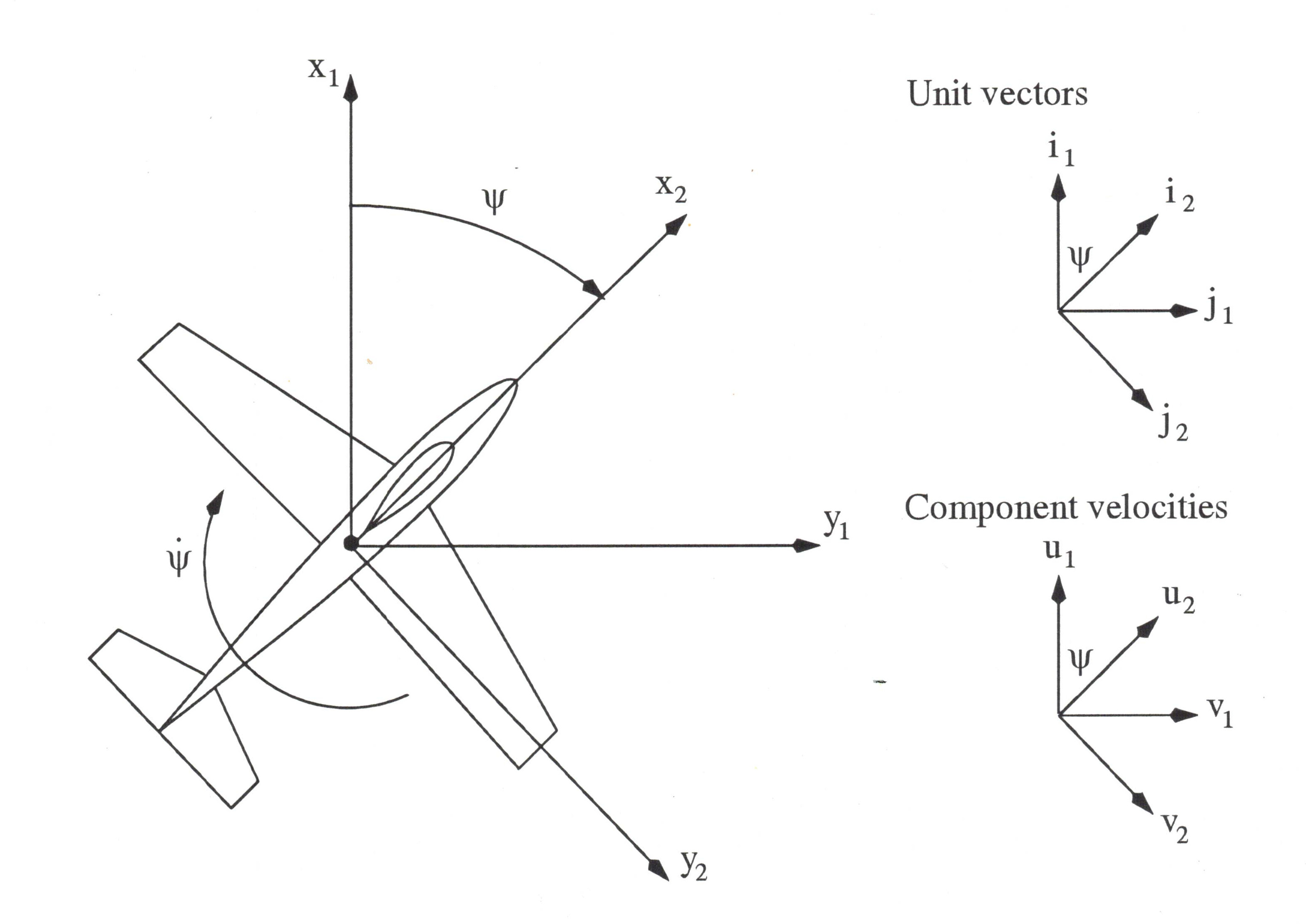 Figure 6(a). Initial Yaw Rotation. 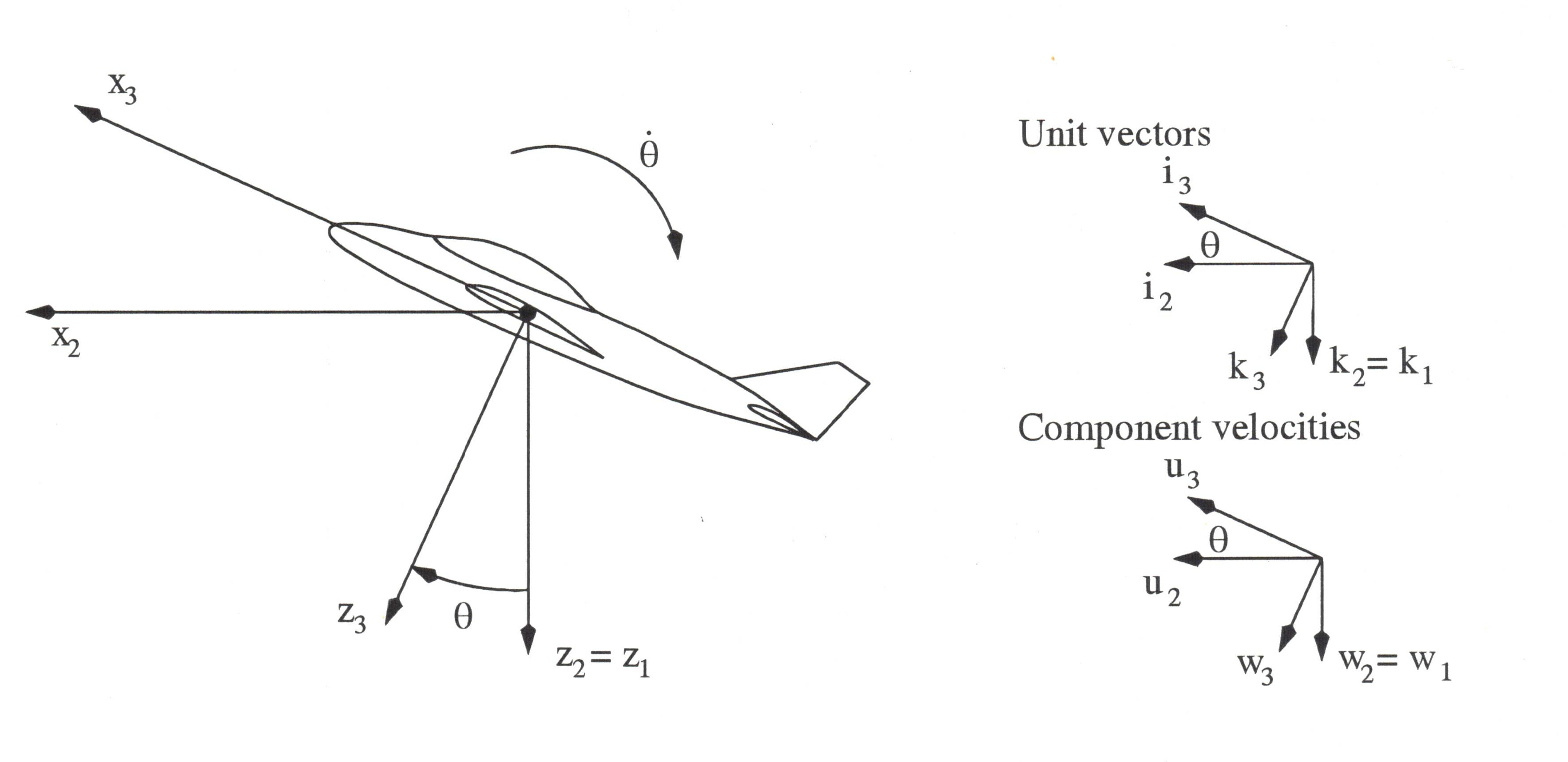 Figure 6(b). Secondary Pitch Rotation. 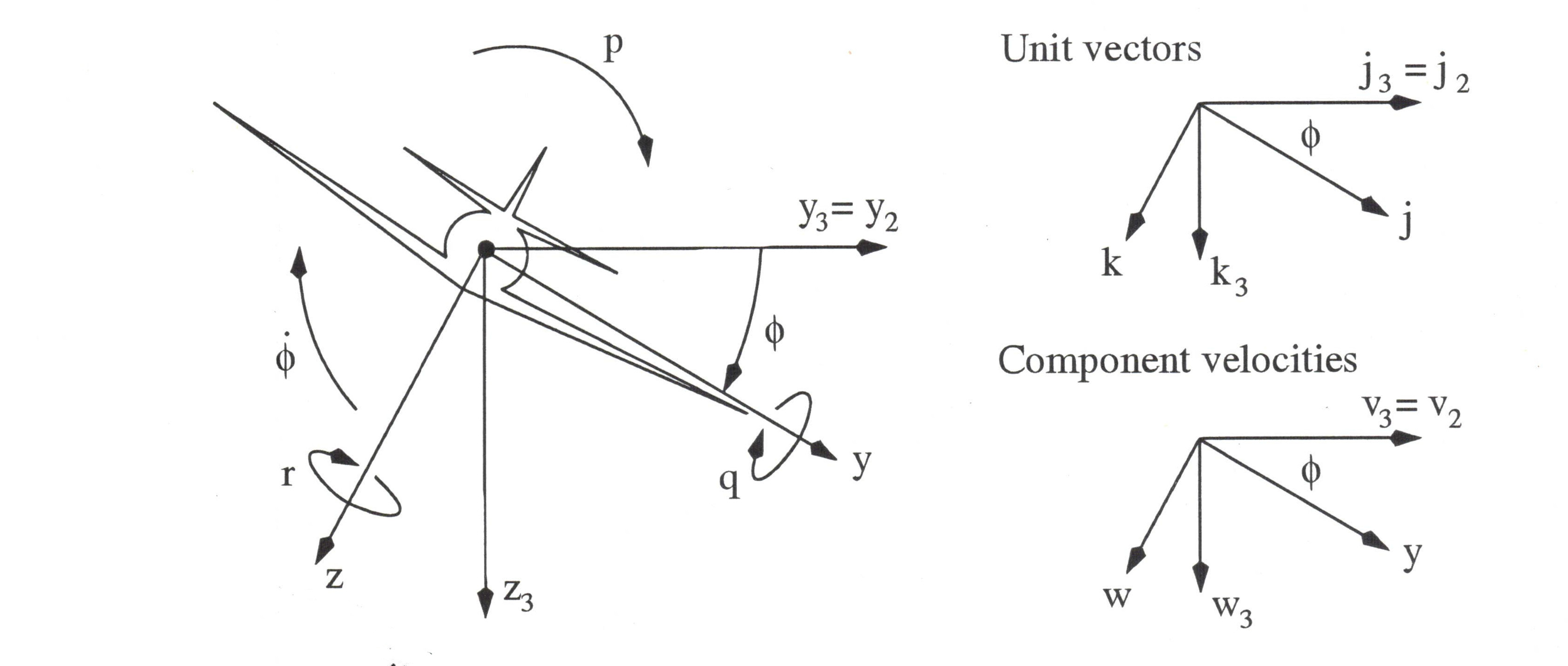 Figure 6(c). Final Roll Rotation. $$ω↖{→}=pi↖{→}+qj↖{→}+rk↖{→}={ψ↖{→}}↖{.}+{θ↖{→}}↖{.}+{φ↖{→}}↖{.}\text" (29)"$$ From the above figures rotation components can be anaylsed to give, $${ψ↖{→}}↖{.}=ψ↖{.}{k↖{→}}_1=ψ↖{.}{k↖{→}}_2$$ $${θ↖{→}}↖{.}=θ↖{.}{j↖{→}}_2=θ↖{.}{j↖{→}}_3$$ $${φ↖{→}}↖{.}=φ↖{.}{i↖{→}}_3=φ↖{.}{i↖{→}}$$ Substituting into Equ. 29 gives, $$ω↖{→}=ψ↖{.}{k↖{→}}_2+θ↖{.}{j↖{→}}_3+φ↖{.}i↖{→}\text" (30)"$$ In order to simplify the analysis, transformations between unit vectors ($i↖{→},j↖{→},k↖{→}$) and ($i↖{→},{j↖{→}}_3,{k↖{→}}_2$) are required. Transformations can be determined from the above Euler angle figures.$${j↖{→}}_3=j↖{→}\cos(φ)-k↖{→}\sin(φ)$$ $${k↖{→}}_3=j↖{→}\sin(φ)+k↖{→}\cos(φ)$$ $${i↖{→}}_2={i↖{→}}_3\cos(θ)+{k↖{→}}_3\sin(θ)$$ $${k↖{→}}_2=-{i↖{→}}_3\sin(θ)+{k↖{→}}_3\cos(θ)$$ In matrix form this can be written as,
Combining this with Equ. 29 gives,
This matrix can be inverted to give Euler angle rates in terms of body axis rotation rates.
Note: Body axes rotation rates and Euler angle rates are not the same. There is also a singularity at $θ=±90^o$. Thus care must be taken using these angles for orientation when the aircraft is in a near vertical climb or descent. Direction CosinesA second method of finding the orientation can be found using aircraft velocity components and how they map from inertial axes frame to the body axes system. Figure 6(a) shows the aircraft velocity components in the earth axes system (1) and the axes system (2) following a yaw rotation $ψ$. Resolving these velocity components gives the relationship,
Similarly, following from Figure 6(b), a rotation from axes system (2) to system (3) through an angle $θ$ gives,
and the final rotation from axes system (3) to the body axes through a roll angle $φ$, gives,
Matrixes $C_1, C_2$ and $C_3$ may be multiplied to give the total rotation of vectors from the inertial frame to the body axes. They can also be used to yield the total rotatations from body axes to the inertial frame as the matrixes are orthogonal and thence their transpose is also their inverse. Therefore, transforming from inertial reference to body axes,
Where $C_{B←E}$ is the transformation matrix from earth to body axes,
Alternately the order of rotations may be reversed in order to transform from body axes to inertial axes,
where
$$C_{E←B}=C_{B←E}^{-1}=C_3^T(ψ).C_2^T(θ).C_1^T(φ)$$
Note: The direction cosines are not restricted for use only with the velocity components, but may be used to transform any vectors between the inertial and the body axes systems. The $C_1, C_2,$ and $C_3$ direction cosine matrices may be applied using appropriate angles to transform vectors between any two axis systems, including body axes, stability axes, wind axes and earth axes systems. A typical application is the transformation of the gravity vector from earth to body axes system,
These transformations may also be used to relate wind axes to earth axes and thus relate the true airspeed to the airspeed components relative to the ground. If earth axis components are defined as $u_1=u_e$, north direction component, $v_1=v_e$, east direction component and $w_1=w_e$, downward component, for no wind conditions, then the required axis transformation will use the heading, $ψ_w$, climb, $θ_w$ and wind axis bank, $φ_w$, angles. In this case the transformation matrix will be,
$$C_{E←W} =C_3^T(ψ_w).C_2^T(θ_w).C_1^T(φ_w)$$
where
and where $V$ is the true airspeed of the vehicle. As true airspeed is aligned with the wind axes, other components $v_w$ and $w_w$ are zero. Note that Equ. 38 only applies to still air conditions. If there is a wind blowing with northerly, $u_{wind}$, easterly, $v_{wind}$ and downward, $w_{wind}$ components, then these will need to be added to the still air solution to give the total velocity of the aircraft with respect to the Earth's surface.
QuaternionsA third method of specifying body orientation relative to an inertial frame is by defining an instantaneous axis of rotation plus a single rotation about that axis.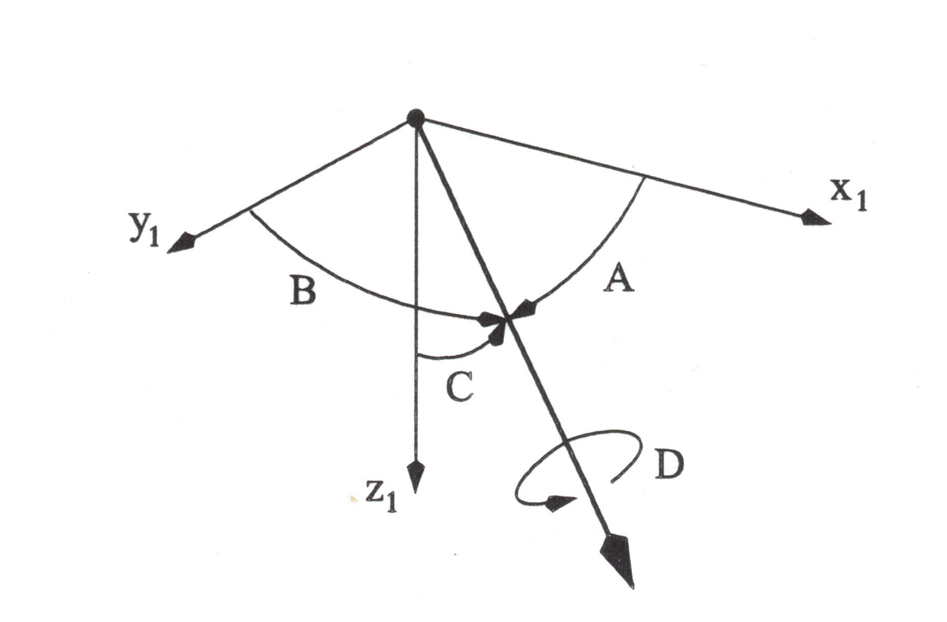 Figure 7. Quaternion relationship between earth and body axes orientations. If the axis of rotation is oriented at angles A,B, and C with respect to the inertial axes ($x_1,y_1,z_1$) as depicted in Figure 7, and the rotation is represented by an angular displacement D, then four quantities $e_0,e_1,e_2$ and $e_3$ can be defined as,
$$e_0=\cos(D/2)$$ These quaternions can be related to Euler angles by,
$$e_0=\cos(ψ/2)\cos(θ/2)\cos(φ/2) + \sin(ψ/2)\sin(θ/2)\sin(φ/2)$$ Their rates of change are related to the body rotation rates as follows:
$${e↖{.}}_0=-1/2(e_1p+e_2q+e_3r)$$ These equations can be used to solve the instantaneous rotations, however it is more useful to obtain them by using the direction cosine matrix and then the Euler angles. Note that the use of quaternions eliminates the singularity problem that occurs when simply using Euler angles. However for a vertical climb or descent the yaw and roll angles will be undefined. Direction cosines were used to relate earth axes and body axes (Equ. 33 and 34) such that
where $l_1$... $n_3$ denote the direction cosines as shown in Equ. 34. They are related to the quaternions as follows,
$$l_1=e_0^2+e_1^2-e_2^2-e_3^2$$ Euler angles can be derived in terms of the quaternions and dirction cosines as follows,
$$θ=\artan({e_0e_2-e_1e_3}/√{(e_0^2+e_1^2-0.5)^2+(e_1e_2+e_0e_3)^2})$$ Any of the three methods (Euler Angles, direction cosines, quaternions) will provide body orientation information. The Euler angles are the most intuitive, but the quaternion method is more robust for digit computation (eg. flight simulators, stability analysis, etc.). Aerodynamic Forces and Wind Axes AnglesThe aerodynamic forces and moments that act on the aircraft are primarily functions of the angle of attack ($α$) and the angle of side slip ($β$). These angles need to be related to the aurcraft body axes so that state and rate variables can be determined. As these aerodynamic angles simply relate the body axes to the wind axes then the direction cosines can be used to obtain the relationship between these two axes systems. Transfering from wind axes to body axes first requires a rotation though $-β$ (side slip angle) about the $z_w$ axis. This is then followed by a rotation through $α$ (angle of attack) (Figure 2). The total rotation can thus be defined using the transform matrix $C_{B←W}$ where $$C_{B←W}=C_1(0).C_2(α).C_3(-β)$$
The body axes velocity components can then be found in terms of the wind axes velocity components as,
The inverse transform gives,
$$V=√{u^2+v^2+w^2}$$ The Equ. 42 can be differentiated using the chain rule to give rates for $V↖{.}$, $β↖{.}$ and $α↖{.}$. However in most flight situations the angles $α$ and $β$ are small so that small angle approximations can be used, $\sin(α)=α$, $\sin(β)=β$, $\cos(α)=1$ and $\cos(β)=1$. Using these approximations and neglecting smaller 2nd order terms, the rate equations are,
$$V↖{.}≈u↖{.}\sec(α)\sec(β)≈u↖{.}$$ Summary of General Equations of MotionBody AxesThe rigid body equations of motion for a symmetric aircraft can be summarised in a body axes reference system as follows: $${\table m(u↖{.}-rv-qw), =, -mg \sin(θ)+F_{Ax}+F_{Tx}; m(v↖{.}+ru-pw), =, mg\sin(φ)\cos(θ) +F_{Ay}+F_{Ty}; m(w↖{.}-qu+pv), =, mg\cos(φ)\cos(θ) +F_{Az}+F_{Tz}; I_{xx}p↖{.}-I_{xz}r↖{.}-I_{xz}pq+(I_{zz}-I_{yy})qr, =, M_{Ax}+M_{Tx}; I_{yy}q↖{.}+(I_{xx}-I_{zz})pr+I_{xz}(p^2-r^2), =, M_{Ay}+M_{Ty}; I_{zz}r↖{.}-I_{xz}p↖{.}+(I_{yy}-I_{xx})pq+I_{xz}qr, =, M_{Az}+M_{Tz}; φ↖{.}, =, p+q\sin(φ)\tan(θ)+r\cos(φ)\tan(θ); θ↖{.}, =, q\cos(φ)-r\sin(φ); ψ↖{.}, =, q\sin(φ)\sec(θ)+r\cos(φ)\sec(θ)} $$
|