Flight Mechanics* General Equations * Linearised Equations * Longitudinal Motion * Lateral Motion * Aerodynamic Derivatives |
Stability of Lateral MotionFor longitudinal motion it was assumed that all disturbances simply moved the aircraft in $u,w$ and $q$, so that there was no motion of the vehicle out of its symmetry plane, ie. $x-z$ axes. In the case of lateral motion the aircraft will move out of the plane undertaking side-slip, $v$, roll $p$ and yaw $r$. For the lateral small disturbance equation solutions, it is assumed that no longitudinal motion is involved at the same time.Neutral Directional StabilityFor longitudinal motion the gravity vector has a significant influence on both static and dynamic stability. For lateral motion this stabilising influence is not present (unless the aircraft has significant asymmetry about the x-z plane), so for lateral motion dynamic stability will dominate except in the case of responses to a disturbance in yaw, $ψ$. While yaw rate, $r$, will be subject to restoring moments to stabilise the motion and attempt to return the vehicle to a trimmed state of $r=0$, the final value of $ψ_f$, the heading of the vehicle, will not be returned to its initial value. Aircraft are neutrally stable in terms of direction or heading, that is, a disturbance will cause the aircraft to set off on a new heading and unless there is a control input it will not return to its original direction with respect to the inertial axes.Dynamic Lateral StabilityIn a similar fashion to the processes for longitudinal stability, a method of finding the free response to a perturbation to the linearised lateral equations of motion will be applied. The assumption is made that the perturbation will simple harmonic motion so the state variables can be defined as,where $v↖{\^}$, $φ↖{\^}$ and $r↖{\^}$ are the peak amplitudes of the motion and $λ$ is the complex frequency. Note: The peak amplitudes can be complex values to allow for magnitude and phase variation, ie. $v↖{\^}=v_R+iv_I$. Also $λ=σ+iω$, a complex value, where $σ$ is the damping or expanding of the motion and $ω$ is the real frequency of the motion. Also in many references an alternate solution is obtained by using state variable $β$ to replace $v$, since due to the assumption of small angles, $β≈v/U$. The time derivative, rates of change of these state variables will be $$v↖{.}=λv↖{\^}e^{λt}\text" , "φ↖{.}=p=λφ↖{\^}e^{λt}\text" , "φ↖{..}=p↖{.}=λ^2 φ↖{\^} e^{λt} \text" , "r↖{.}=λr↖{\^}e^{λt}$$ Substituting these harmonic variables into the lateral perturbation equations gives, $$v↖{\^}e^{λt}(−L_v)+φ↖{\^}e^{λt}(λ^2−λL_P)+r↖{\^}e^{λt}(−λ{I_{xz}}/{I_{xx}}-L_r)=L_{δ_a}δ_a+L_{δ_r}δ_r$$ $$v↖{\^}e^{λt}(−N_v)+φ↖{\^}e^{λt}(-λ^2{I_{xz}}/{I_{zz}}-λN_p)+r↖{\^}e^{λt}(λ−N_r)=N_{δ_a}δ_a+N_{δ_r}δ_r$$ If looking for the free response of the aircraft for lateral motion, the perturbation control deflections can be set to zero. So that the free response system becomes, $$v↖{\^}e^{λt}(λ−Y_v)+φ↖{\^}e^{λt}(−λY_p−g)+r↖{\^}e^{λt}(U-Y_r)=0$$$$v↖{\^}e^{λt}(−L_v)+φ↖{\^}e^{λt}(λ^2−λL_P)+r↖{\^}e^{λt}(−λ{I_{xz}}/{I_{xx}}-L_r)=0$$ $$v↖{\^}e^{λt}(−N_v)+φ↖{\^}e^{λt}(-λ^2{I_{xz}}/{I_{zz}}-λN_p)+r↖{\^}e^{λt}(λ−N_r)=0$$ This system can be written in matrix format,
where $k_1=I_{xz}/I_{xx}$ and $k_2=I_{xz}/I_{zz}$ As was the case for longitudinal motion, a free response solution for lateral motion will either be a simple, zero motion, stable solution, $v↖{\^}=φ↖{\^}=r↖{\^}=0$ or a set of frequency responses when |[.]|=0. The determinant of the matrix can be expanded in terms of $λ$ such that
where $$p_4=1-k_1k_2$$$$p_3=-L_p-N_r-Y_v-k_1N_p-k_2L_r+k_1k_2Y_v$$ $$p_2=L_pN_r-N_pL_r+L_pY_v+N_rY_v-L_vY_p-N_vY_r+k_1N_pY_v+k_2L_rY_v-k_1N_vY_p+k_2UL_v-k_2L_vY_r+UN_v$$ $$p_1=-L_pN_rY_v+N_pL_rY_v+L_vN_rY_p-L_rN_vY_p-N_pL_vY_r+L_pN_vY_r-gL_v-gk_1N_v+UN_pL_v-UL_pN_v$$ $$p_0=gL_vN_r-gL_rN_v$$ Note: In many cases the scaled products of inertia, $k_1$ and $k_2$ are small and neglected in the above equations. In any case the solution of the quatic equation results in 4 roots, typically 2 real roots and 1 complex pair, 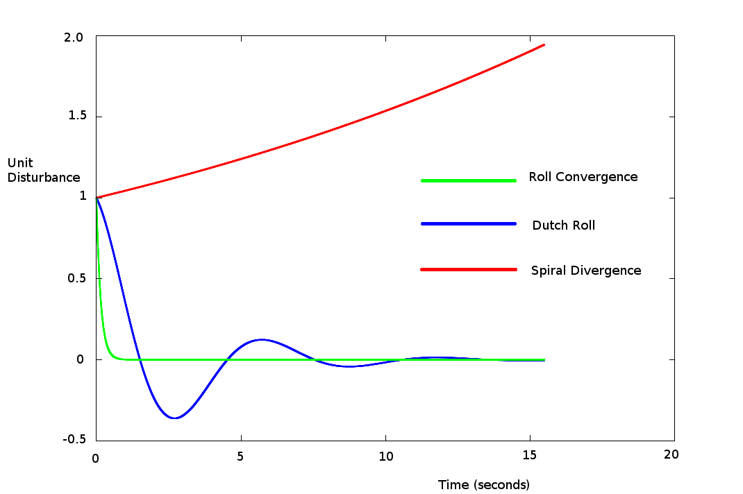 Figure 1. Free Response lateral modes of motion for a transport aircraft Roll ConvergenceOne of the solutions for the lateral quartic equation will be a real large negative root. This is a response to a roll rate disturbance which would produce a large differential in the lift on either wing. The upgoing wing experiences reduced lift, the down going wing experiences increased lift and this produces a strong stabilising moment to stop the rate of roll. Note however, that this does not necessarily have a significant affect on the roll angle and other factors are required to restore $φ$ to its original trimmed state.A simplifying approximation of this result can be obtained by assuming no side-slip or yaw affects which mean the motion is dominated by the central term from the roll equation from the full lateral equations of motion. hence where $L_p$ is typically in the range $L_p<-0.25$ (low aspect ratio wings), $-6<L_p$ (high aspect ratio wings). Spiral ModeThe second real root of the quatic tends to be small but could be either positive or negative. This results from a yaw disturbance coupled with a small roll angle disturbance (clockwise). In many cases, without other stabilising affects such as dihedral, this motion leads to increased side-slip and the aircraft enters an unbalanced turn. The increase in drag and slight reduction in lift in this situation would mean that the motion cause the aircraft to enter into a descending spiral. The rate of change is small so if the spiral mode is unstable, the motion can be corrected by the pilot or by an automatic wing leveling device. An approximate result for this mode can be found by assuming λ is small and thus neglecting the smaller higher order terms in the equation, $$λ=-{p_0}/{p_1}$$ This can be further simplified by assuming the smaller lateral aerodynamic derivatives and the scaled products of inertia are negligible, ie. $Y_p≈Y_r≈k_1≈k_2≈0$. Dutch Roll ModeThe complex pair of roots lead to a motion called Dutch Roll. It is an oscillatory motion combining roll, yaw and side-slip. The roll and yawing motions are out of phase, so unlike the spiral mode which can cause divergent behaviour, this mode causes a damped rocking motion of the aircraft. The frequency of motion tends to lie between the values of the longitudal short period mode and phugoid mode. If this mode is only lightly damped it can detract from the handling qualities of the aircraft. The Dutch Roll motion entails reasonable yaw $r$ and side-slip $v$ rates but only small roll rates $p$. So a simplified solution can be obtained by analysing the lateral motion without roll rate valiables. ie.,
Again setting the determinant of the matrix to zero will lead to an approximate solution in the form of a quatratic equation. where $$p_0=N_rY_v-N_vY_r+N_vU$$ and |