Fluid Mechanics

Fluid Statics

Fluid statics and fluid dynamics form the two constituents of fluid mechanics. Fluid statics deals with fluids at rest while fluid dynamics studies fluids in motion. In this section fluid statics is covered.

A fluid at rest has no shear stress. Consequently, any force developed is only due to normal stresses i.e, pressure. Such a condition is termed the hydrostatic condition. In fact, the analysis of hydrostatic systems is greatly simplified when compared to that for fluids in motion.

Though fluid in motion gives rise to many interesting phenomena, fluid at rest is by no means less important. Its importance becomes apparent when it is noted that the atmosphere around us can be considered to be at rest and so are the oceans. The simple theory developed here finds its application in determining pressures at different levels of atmosphere and in many pressure-measuring devices. Further, the theory is employed to calculate force on submerged objects such as ships, parts of ships and submarines. Other applications of this theory are used in the calculation of forces on dams and other hydraulic systems.

Fluid Forces

In fluid mechanics forces upon fluid elements need to be considered. These forces can be divided into two categories - Surface Forces, F_s and Body Forces, F_B.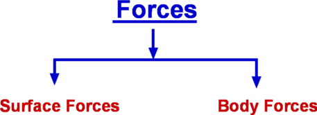

Figure 1 : Classification of forces

Surface forces are brought about by contact of fluid with another fluid or a solid body. The best example of this is pressure. The surface forces depend upon surface area of contact and do not depend upon the volume of fluid. On the other hand, body forces depend upon the volume of the substance and are distributed through the fluid element. Examples are weight of any substance, electromagnetic forces etc.

Pressure at a point within a fluid

Considering a fluid at rest as shown in Fig. 2, at the point of interest, P, a small wedge of dimensions dx x dz x ds can be defined. Let the depth normal to the plane be b. In this derivation, z is the vertical coordinate. This is consistent with the use of z as the elevation or height in many applications involving atmosphere or ocean. Surface forces and body forces acting on the wedge are also indicated in the diagram.

The surface forces acting on the three faces of the wedge are due to the pressures, P_x, P_z and P_n as shown. These forces are normal to the surface upon which they act. Compressive pressure is assumed to have a positive sign. Since the fluid is at rest there is no shear force acting.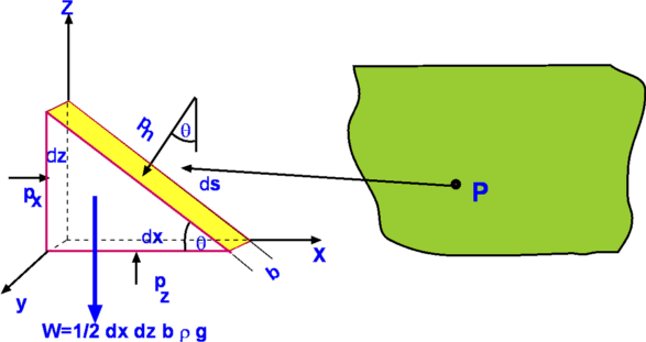

Figure 2 : Pressure at a point

In addition there is a body force, the weight, W, of the fluid within the wedge acting vertically downwards. Summing the horizontal and the vertical forces we have,

or

Note that

thus, after simplification,

Note that the pressure in the horizontal direction does not change, which is a consequence of the fact that there is no shear in a fluid at rest. In the vertical direction there is a change in pressure proportional to density of the fluid, acceleration due to gravity and difference in elevation.

Now if we take the limit as the wedge volume decreases to zero, i.e., the wedge collapses to the point P, we have,

This equation is known as Pascal's Law. It is important to note that it is valid only for a fluid at rest. In the case of a moving fluid, pressures in different directions could be different depending upon fluid accelerations in different directions. Hence, for a moving fluid, pressure is defined as an average of the three normal stresses acting upon the fluid element.

Equation for Pressure Field

For a fluid at rest the pressure at any point is invariant with direction. However, this does not prevent pressure itself varying from point to point within the fluid. In this section a relationship for variation of pressure is established.

A rectangular element of fluid of dimensions dx x dy x dz with centre at the point P(x,y,z) is shown in Fig. 3. Let the pressure acting at the point P be equal to P. It is then assumed that pressure varies continuously across the element.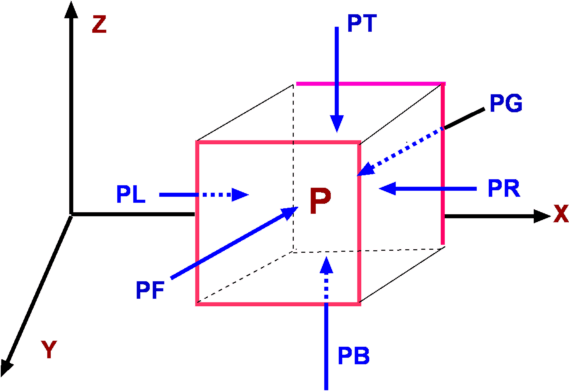

Figure 3: Components of pressure at a point

The pressures at the different faces of the element are calculated by expanding pressure in a Taylor series about point P. Linear gradients are assumed for this very small element and second and higher order terms are neglected. Accordingly,

A surface force balance in the x-direction gives

Similar force balancing is carried out in each of the other directions. Upon collecting terms, the result for surface forces acting on the fluid element is,

The terms within the parenthesis is called the pressure gradient. i.e.,

Thus,

The net surface force upon the element is given by the pressure gradient and is not dependent upon the pressure level itself.

Body Forces

The only body force is the weight of the fluid element or the gravity force.

Total Force

Adding the surface and body forces acting on the fluid element, gives the total force,

On a per unit volume basis this equation becomes

Thus an expression for force upon a unit volume of a fluid element at rest has been derived. To extend this to the case of a moving fluid, normal and shear stresses due to viscosity must be included in addition to the forces given above. For a fluid at rest, the net force should be equal to zero. Accordingly,

The above equation consists of three separate equations, one for each direction and each of them must be equal to zero. Thus for x, y and z directions we have,

If the coordinate system be so selected as to align one of x, y or z with acceleration due to gravity, g the equations simplify considerably. The natural selection is to have z-direction align with -g, such that g_z = - g. Consequently, g_x = g_y = 0. Then,

The above equation shows that pressure in a static fluid does not vary in x or y direction. It varies only in the z-direction. This can be writen,

The above equation is a fundamental governing equation for fluid statics. It defines the manner in which pressure varies with height or elevation and is used in many different applications. It enables determination of atmospheric pressures at different elevations above the sealevel or the pressure variation in the depths of the ocean. Another application is in Manometry, which forms the basis of a class of pressure measuring instruments.

The equation reveals that the pressure gradient is a function of density, ρ and acceleration due to gravity, g . Gravity, g is almost a constant and therefore it is the variation in density with elevation that influences the pressure values. Density is constant for incompressible fluids and varies with pressure and temperature for compressible fluids. Therefore it is necessary to consider these two types of fluids separately.

Incompressible Fluids

For incompressible fluids density is a constant. In addition, for most applications of practical interest, acceleration due to gravity is also a constant. As a consequence the pressure equation is greatly simplified and can be readily integrated. Thus for incompressible fluids,

which on integration yields

A convenient arrangement of the above equation is

where h is the difference in elevation, z₂ - z₁.

By rewriting the above equation, we have,

These equations demonstrate that pressure difference between two points in an incompressible fluid is proportional to the difference in elevation or height between the two points. The term h is sometimes defined as the pressure head and is the height of the fluid column of density, ρ, (or specific weight, γ ) that is supported by a pressure difference of ( P₁ – P₂ ).

The above can be used to determine pressures in atmosphere and ocean depths. For this application, a convenient datum or reference needs to be chosen. Depending upon the application, sea-level (for atmospheric pressure) or free surface (for measurements in oceans and lakes) is ideally suited.

For an ocean or a lake, if P_a is the pressure acting on the free surface pressure at any depth h₂ is given by

For the atmosphere with P_a being the sea level pressure,

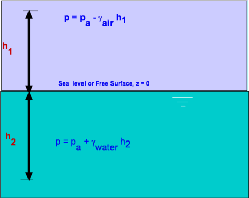Figure 4 : Measurement of pressure in atmosphere, oceans and lakes.

However, care should be taken only to apply this to small distances in air as air is compressible and over large heights, other effects dominate.

Compressible Fluids, Properties of Atmosphere

The most common compressible fluid we know is air. Assuming air to behave like a perfect gas, the hydrostatic equation becomes,

or

By integrating the above equation,

To solve the above equation, the variation of temperature T with altitude must be determined. This information and the subsequent solution is shown in the following section on Standard Atmosphere Properties.

Measurement of Pressure

Another application of the equation of fluid statics is for devices used to measure pressure. Pressure is measured as either an absolute pressure or a gauge pressure. Pressure is always measured as a difference with respect to a datum or reference. Absolute pressure is measured relative to a perfect vacuum, whereas gauge pressure is measured relative to surrounding atmospheric pressure. Further, absolute pressure is the sum of atmospheric pressure and the gauge pressure.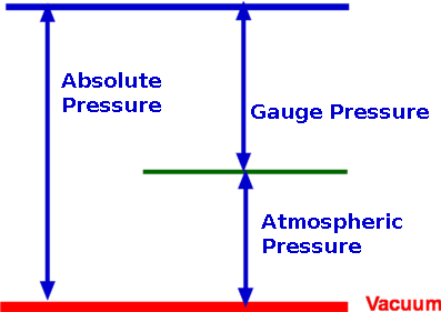

Figure 8 : Definition of gauge and absolute pressures

Manometry

Pressure is proportional to the height of a column of fluid. Manometry exploits this to measure fluid pressure. By measuring the height of a column of liquid supported by the pressure difference, it is possible to infer the value of pressure. Barometer, piezometer and U-tube manometer are some of the members of this class of instrument.

Mercury Barometer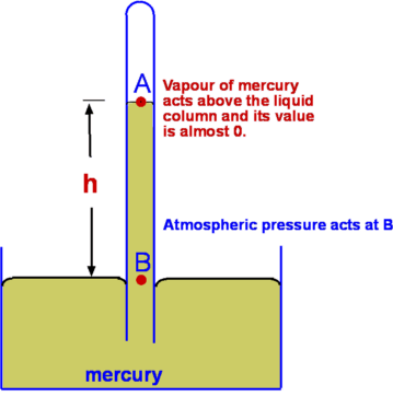

Figure 9 : Mercury Barometer

Mercury Barometer (Fig.9) is the simplest device to measure atmospheric pressure at a location. It consists of an evacuated glass tube closed at one end immersed in a container filled with mercury. Because of the atmospheric pressure mercury rises in the tube as shown. If h is the height of mercury above the fluid level in the container, then

Where P_A is the pressure at A and will be equal to the vapour pressure of mercury, P_vap, which is around 0.16pa at a temperature of 20^oC. It is usual to neglect P_A as it is quite small, then atmospheric pressure is given as

Sometimes atmospheric pressure is expressed as "mm of mercury" which is the measure distance h. At standard sea level conditions, the pressure value is 101,327 Pascals and the specific weight of mercury is 133,100 N/m³, the barometric height is 761 mm Hg. Water could be used as the barometer fluid, but in that case the height of water would be around 10.36 m!

Piezometer Tube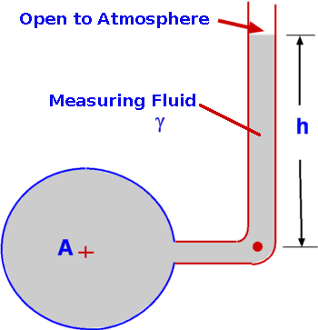

Figure 10 : Piezometer

Piezometer tube (Fig. 10) is another simple pressure measuring device and consists of a vertical tube. In this application one end is connected to the pressure to be measured while the other end is open to the atmosphere as shown. Application of hydrostatic equations gives

or simply for the gauge pressure at A,

U-tube Manometer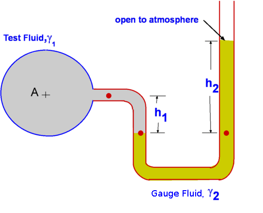

Figure 11 : U Tube Manometer

Although the piezometer tube is simple in structure, it has a few practical disadvantages. The U-tube Manometer (Fig. 11 is a better alternative. It is a U-tube filled with what is called a gauge fluid. As before one end of the tube is exposed to the pressure to be measured while the other end is open to atmosphere.

or as a gauge pressure

Considerable simplification is possible if the fluid A is a gas where $ γ_1 h_1 $ is negligible in comparison to the gauge fluid, giving

Differential U-tube Manometer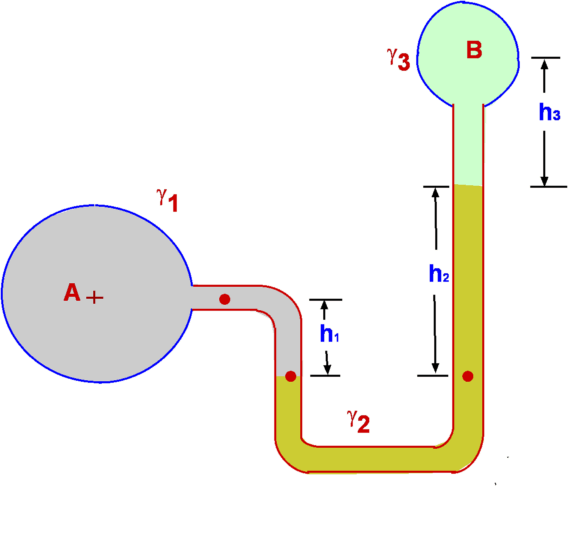

Figure 12 : Differential U-tube manometer

Differential U-tube manometer (Fig. 12) is used to measure the pressure difference directly and is basically similar to the U-tube manometer discussed above. What was the open end before is now connected to a different pressure, P_B so that the difference P_A – P_B is now measured. Thus,

so that

Hydrostatic Force on a submerged surface

Another important use of the hydrostatic equation is in the determination of forces acting upon submerged bodies. Among the innumerable applications of this are the force calculation in storage tanks, ships, dams etc.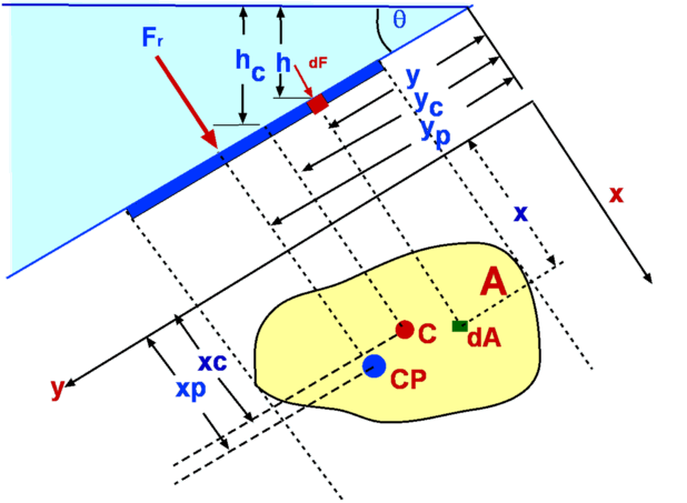

Figure 13 : Force upon a submerged object

First consider a planar arbitrary shape submerged in a liquid as shown in Fig. 13. The plane makes an angle θ with the liquid surface, which is a free surface. The depth of water over the plane varies linearly. This configuration is efficiently handled by prescribing a coordinate frame such that the y-axis is aligned with the submerged plane. Consider an infinitesimally small area ΔA=dx.dy at (x,y). This small area is located at a depth h from the free surface. From hydrostatic equation,

Where P is the pressure acting on the free surface. The total hydrostatic force on the plane is given by,

The integral, $ ∫ y dA $ is the first moment of area about the x-axis. If y_c is the y-coordinate of the centroid of the area then,

Consequently, this can be rewritten as

where $ h_c = y_c \sin(θ)$ and P_C is the pressure acting at the centroid.

Centre of Pressure

Force, F, is the resultant force acting on the plane due to the liquid and acts at what is called the Center of Pressure (CP). It does not act at the centroid of the plane as could be infered from the above calculation. Assume the coordinates of CP are (x_p,y_p). The moment of the resultant force is equal to the moment of the distributed force about the same axis, so that

Before substituting for F in the above equation, note that the atmospheric pressure P_A >acts at the free surface and is also distrubuted everywhere within the fluid as a constant, so it is constant on both sides of the x-axis or y-axis. As such, it does not contribute to the net force or moments upon the plane. P_A will be dropped from the equation for F. The equation for moments bout the x-axis becomes,

The term $ ∫_A y^2 .dA $ is the second moment of area about the x-axis denoted by I_xx leading to

I_xx is measured about the x-axis. If I_xc is defined as the second moment of area about the centroid (x_c,y_c) then through the Parallel Axes Theorem the relationship between second moments of area can be found,

Consequently,

Similarly, taking moments about the y-axis, we obtain,

Leading to

I_xy is the product of inertia with respect to x and y axes. Again on the application of the parallel axis theorem we have

Where I_xyc is the product of inertia about the axes passing through the centroid. The coordinates of the centre of pressure are thus given by (x_P,y_P) .

The resulting force upon the immersed surface is therefore given by

The centre of pressure is given by

Expressions for the moments I_xc, I_xyc for some of the common shapes are given in the next section.

Geometrical Properties of Common Shapes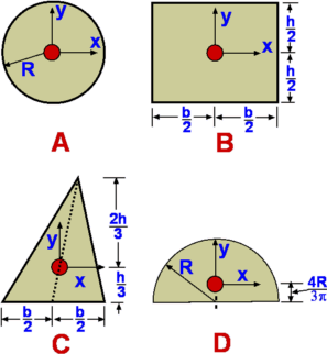

Figure 14 : Properties of some common shapes

Note that the determination of the resultant force F_R is based on the knowledge of the position of the centroid for the given shape. The location of CP, the center of pressure depends upon the moment of inertia and the product of inertia.

These are functions of the geometry only and can be calculated once the shape is given. The above Table along with Fig. 14 gives these properties for some of the common shapes.

Hydrostatic Force on a Curved Surface

We encounter many arbitrarily shaped bodies immersed in liquids such as pipes and walls of containers. Forces on these may be calculated in the same manner as in the previous section. But the required integration of involved terms becomes very tedious. A more simplistic approach is to consider the forces resolved in the three coordinate directions separately. It may be noted that each component of force acts upon a projected area of the body. For example, force in x-direction will act normally on the area projected upon the y-z plane.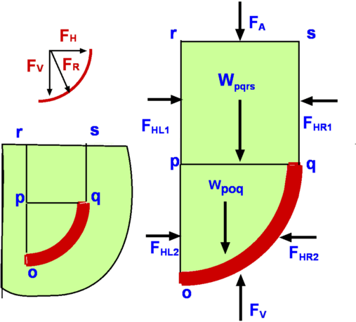

Figure 15 : Hydrostatic forces on a curved surface

Consider a curved surface as shown in Fig.15, immersed in a liquid. The resultant force F_R can be resolved into two components - F_H in the horizontal direction and F_V in the vertical direction. We are considering a thin body which is two-dimensional and as such there is no force in the direction normal to the plain. The configuration can be split into two parts; 1: the part between the body and the free stream , pqrs and 2: the body itself, poq. Consider each part separately.

Block of fluid pqrs is in equilibrium. The horizontal forces acting on it cancel out. Thus,

Similarly on the block poq we have,

The horizontal F_HL2 can be estimated by integrating pressure over the depth of this side. The vertical forces acting upon the fluid are (1) F_A due to atmosphere, (2) W_pqrs, the weight of block pqrs and (3) W_poq, the weight of block poq. Consequently,

Force F_A is given by the atmospheric pressure times the projected area normal to it. The resultant force, F_R is given by,

Buoyancy and Stability

To find the vertical force acting on a body which is completely submerged in a fluid, the theory developed above can be applied. What is known as Archimedes principle states -

1. The vertical buoyant force experienced by a body immersed in a fluid is equal to the weight of the fluid displaced.

2. A floating body displaces its own weight of the fluid.

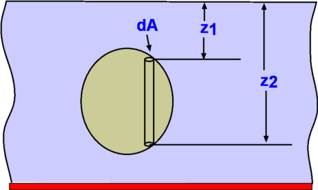Figure 16 : Forces about a body immersed in a fluid (part 1)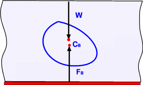



Figure 17 : Forces about a body immersed in a fluid (part 2)

The proof of these rules is relatively straight forward. Consider an elemental volume within the immersed body as shown in Fig. 16. The buoyant force is given by,

where dA is the area of cross section of the elemental volume. Thus,

It can be shown that the buoyant force, F_B passes through the centroid of the displaced volume as shown in Fig. 17. The point where this force acts is called the Center of Buoyancy and is denoted as CB

The above result holds even in the case of a partially submerged body i.e., a floating body. It is assumed that part of the body above the liquid level is in air. The weight of air displaced as a consequence is ignored. (Fig. 18). For this case as well,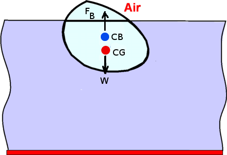

Figure 18 : Partially Submerged Body

The theory developed so far also aplies in case of a fluid for which specific gravity, γ is not a constant, for example, a layered fluid. However in this case, the buoyancy force may not act at the centroid of the displaced volume.

The theory developed is also applicable where the fluid involved is a gas, eg. air. Convection currents established in atmosphere depend upon the buoyancy forces generated.

Stability of Immersed and Floating Bodies

Stability becomes an important consideration when floating bodies such as a boat or ferry are designed. It is an obvious requirement that a floating body does not topple when slightly disturbed. A body is in stable equilibrium if it is able to return to its original position when slightly disturbed. Failure to do so denotes an unstable situation and the motion will be magnified not reduced. Whether a floating or submersed body is stable is decided by the couple formed by the weight of the body and the buoyancy force. Consider the immersed body shown in Fig.19. In general, if the center of gravity of the body lies below the center of buoyancy stable equilibrium prevails. An overturning couple leading to unstable motion results if the center of gravity is above the center of buoyancy (Fig. 20).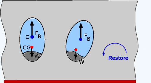

Figure 19 : Stability of an immersed body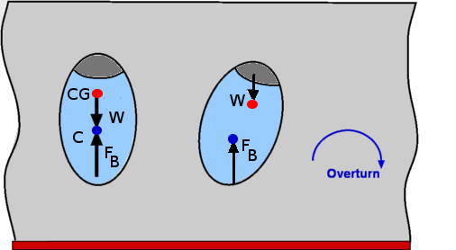



Figure 20: Instability of an immersed body

The problem becomes more complicated when floating bodies are considered. As the body rotates responding to any disturbance, the center of buoyancy can shift. This could render the body stable even though the center of gravity is above the center of buoyancy. This is particularly true of the bodies with a broader base such as a barge (Fig. 21). A slender body as shown in Fig. 22 is very susceptible to instability.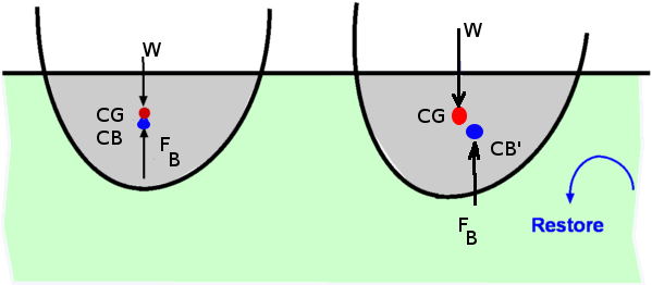

Figure 21 : Stability of a floating body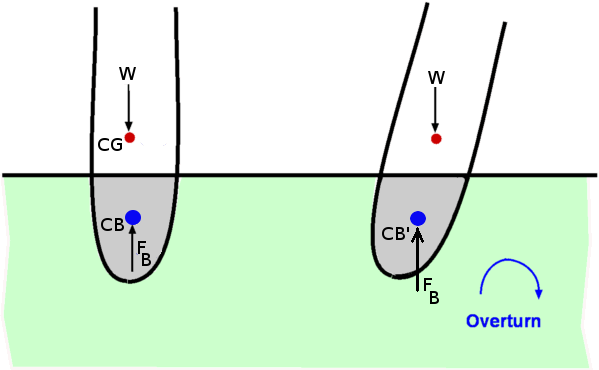



Figure 22 : Instability of a floating body