Fluid MechanicsProperties of Fluids Fluid Statics Control Volume Analysis, Integral Methods Applications of Integral Methods Potential Flow Theory Examples of Potential Flow Dimensional Analysis Introduction to Boundary Layers Viscous Flow in Pipes |
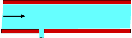
Applications of Integral Conservation EquationsThe Bernoulli equation is one of the most useful equations in fluid mechanics and finds many applications. In many cases, the equation is used in devices for the measurement of fluid flow. One such case is the measurement of flow by introducing a restriction within the flow. The restriction may take the form of an orifice plate or a converging-diverging nozzle. Flow through a Sharp-edged OrificeAn orifice plate placed in a pipe flow is shown in Fig 1. It is assumed that the thickness of the plate is small in comparison to the pipe diameter. The orifice is assumed to be sharp edged so that separation effects of a rounded plate will not need to be considered here. 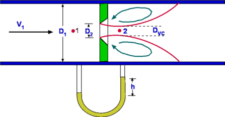 Figure 1: Flow through an Orifice Body A fully developed flow prevails at the upstream of the orifice. The presence of the orifice causes the flow to accelerate through it thus increasing the velocity. The flow will separate from the sharp edges and take a length of pipe to return to a fully developed flow covering the complete area. A slow moving recirculating flow develops behind the plate. This recirculating mass of fluid acts as an obstruction in the flow and forms a curved bounday between the slow moving mass and the fluid coming through the orifice. As a consequence the smallest diameter of flow is not equal to the orifice diameter, but slightly smaller and at a position downstream of the orifice.(2) The flow rate through the pipe can be predicted by measuring the pressure difference upstream of the plate compared to that behind the plate in the recirculating zone. A few assumptions about the flow are made,
The equations applied are (a) Continuity and (b) Bernoulli equations. a) Continuity Equation. b) Bernoulli Equation The Bernoulli equation gives, Noting from Continuity that then Solving for V2 gives, Consequently, the mass flow rate becomes, $${dm}/{dt}=A_2/{√{1-(A_2/A_1)^2}}√{2ρ(P_1-P_2)}$$ The above equation gives the mass flow rate through the pipe in terms of the pressure drop and the areas. The equation gives only a theoretical value. In order to obtain a more realistic value the actual area at the minimum cross section (2) or the Vena Contracta needs t be found and used in the calculation. In addition losses may not be negligible. The extent of losses is a function of the Reynolds number. In practice, a Coefficient of Discharge, C is defined such that, Further if we define a ratio of diameters β such that $${dm}/{dt}={CA_2}/{√{1-β^4}}√{2ρ(P_1-P_2)}$$ Sometimes the ratio $1/{√{1-β^4}}$ is referred to as Velocity of Approach Factor. Again it is usual to combine this and the Discharge Coefficient to define a Flow Coefficient given by Consequently the mass flow rate is given by, Thus the mass flow rate for a pipe can be calculated with the knowledge of pressure drop, the orifice diameter and the coefficient K. Extensive measured data exists in handbooks for the coefficient K for differing orifice sizes. Pressure drop is usually measured by using a manometer as shown in Fig 1. The pressure drop is obtained as h, the height of a liquid column. Accordingly, where γ is the specific weight of the manometer fluid. Flow Through a Nozzle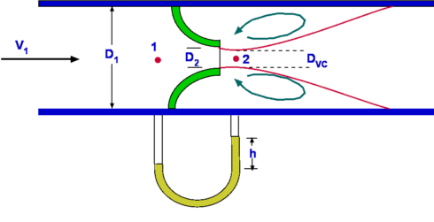 Figure 2 : Flow through a Nozzle Though geometrically different from an orifice plate, a flow nozzle is conceptually similar to it. Fig 2. shows a flow nozzle which is just a converging nozzle placed in a pipe. The flow mechanism is similar to that for the orifice. The area A2 is the throat area of the nozzle and is better defined than for the orifice. Flow through a Venturi Tube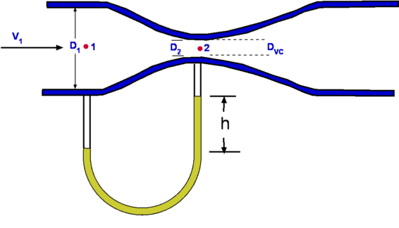 Figure 3: Venturi Tube A Venturi Tube is a converging-diverging nozzle, Fig.3., placed in a pipe. The principle of this was demonstrated by Giovanni Battista Venturi (1746-1822) in 1797. It was only later in 1887 that it was employed for flow measurement by Herschel. The mass flow rate is given by the above equation. In this case the correction factor due to losses is almost 1.0 Applications of Control Volume AnalysisIn this section applications of the control volume analysis are considered. Each analysis relies to some extend on the the equations of continuity, momentum and energy. Measurement of Drag about a Body immersed in a fluidConsider a body such as an aerofoil placed in a flow such as a wind tunnel. Far from the body the flow is uniform and inviscid. As the flow approaches the body, many changes take place. The flow will start to depart from uniformity. For the flow region surrounding and downstream of the body viscosity comes into play. Consequently, the velocity on the body surface is zero. The velocity catches up with the freestream speed as we move away from the body. In other words, a boundary layer develops. A boundary layer is not static. It grows as the flow moves downstream. When the flow leaves the body the centreline velocity is not zero as the flow mixes in the wake region. It starts to build up slowly. If a velocity profile is measured across the wake by carrying out what is called a Wake Traverse, then a result as shown in Fig.4 is obtained. The wake profile thus carries signatures of the viscous effect on the flow of the presence of the aerofoil upstream. 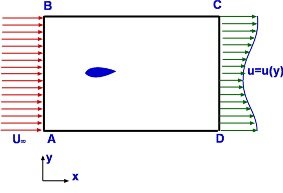 Figure 4: Measurement of Drag about an immersed body If a momentum balance is conducted in a region surrounding the aerofoil then a force imbalance is evident. This is equivalent to the drag exerted on the aerofoil by the stream. To undertake the analysis a control volume ABCD is selected. The left and right hand boundaries AB and CD are far from the body. The flow is uniform ( at a speed $U_{∞}$) on AB. At the right hand boundary, CD, is the wake with the velocity profile as shown, equal to freestream at the edges but with a deficit in the center. It is assumed that the top and bottom boundaries of the control volume, AD and BC are far away from the body and the vertical component of velocity, v, is zero across them. The following assumptions are made,
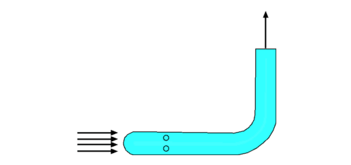
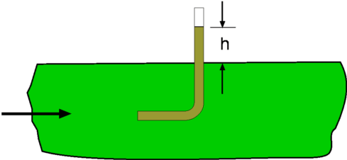
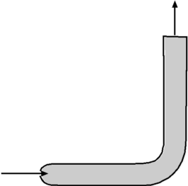
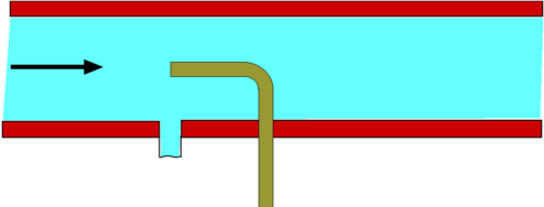
Continuity Equation.Since the flow is steady, i.e., since vertical component of velocity along BC and DA is zero, the equation reduces to The flow is assumed to be purely horizontal at inlet and outlet, V = u, with incoming massflow on the inlet and outgoing massflow on the outlet then, thus Momentum equationOn applying the momentum equation to the control volume, the x-direction component can be found as, since v = 0 on BC and AD, At inlet V = constant = $U_{∞}$ , at outlet V = local horizontal velocity = u. Applying the result from the continuity equation gives, The body force FBx on the control volume is zero. The surface forces are a reaction force to stop the aerofoil moving, ie. drag reaction,FSx=D, and the pressures on the boundaries. Since it is assumed that pressure is uniform, the latter is zero. As the flow can be assumed to be two-dimensional with a unit depth, then dA = 1.dy. If the top and bottom of the tunnel are assumed to be far from the aerofoil and wake then the final result becomes, Inaccuracies arise in the above analysis due to top and bottom wall friction effects which will cause a pressure drop between the inlet and outlet. Another method is to make these boundaries streamlines of flow. This allows the control volume to grow between AB and CD so that there is no wall losses involved. Then $AB≠CD$. Jet Impingement on a surfaceConsider a jet with a cross section Aj at a speed Vj impinging on a solid surface at an angle θ as shown in Fig 5. It is required to calculate the normal force exerted on the surface. 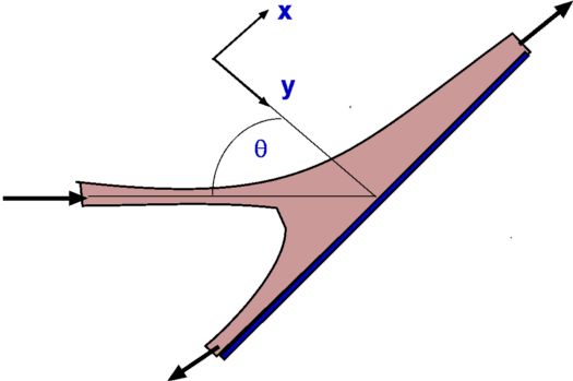 Figure 5 : Jet impinging on a surface As the jet impinges upon the surface, it splits into two parts. These move tangential to the surface. The normal component of the force acting upon the surface needs to be resisted by a reaction force otherwise the plate will move. Define x and y axes parallel and perpendicular to the surface as shown and chose a control volume surrounding the fluid and cuting through inlet and outlet streams. At the entry to the control volume we have the momentum in the y-direction equal to At the solid surface where the flow exits the control volume, the velocity normal is zero and as such there is no normal momentum acting. Assuming the pressure is uniform around the outside of the stream means that the above change in momentum is equal to the normal force acting upon the surface. Force on a Pipe BendConsider a flow through a pipe bend as shown. The flow enters the bend with a speed V1 and leaves it a speed V2, the corresponding areas of cross section being A1 and A2 respectively. The velocities have components u and v in x and y directions. It can be assumedn that the flow is uniform over the inlet and outlet faces. As the flow negotiates the bend it exerts a force upon it. This force is readily calculated by the momentum theorem. 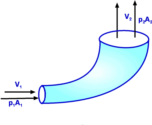 Figure 6: Force on a Pipe Bend The continuity equation yields Carrying out a force balance in x-direction, we have $$P_1A_1-P_2A_2\cos(θ)+F_x={dm}/{dt}V_2\cos(θ)-{dm}/{dt}V_1={dm}/{dt}(V_2\cos(θ)-V_1)$$ In the y-direction we have, giving Thus the force components acting on the bend are $$F_y=P_2A_2\sin(θ)+{dm}/{dt}V_2\sin(θ)$$ Froude's Propeller TheoryPropellers are a mechanism for the propulsion of an aircraft. In its generic form, a propeller is pair of rotating blades mounted on a shaft connnected to an engine. As the engine operates the propeller turns sucking in a large amount of air. As this air passes through the rotating blades, it gets energised, its speed increases. In the process the momentum change produces the required thrust to propel the aircraft. 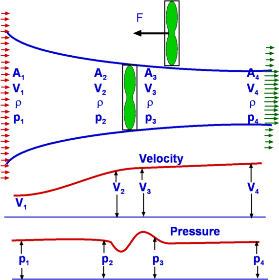 Figure 7: Froude analysis of a Propeller The propeller is modelled as as a thin disc rotating in air as shown in Fig 7. The pressure and velocity far away from the disc i.e., at section (1) are P1 and V1 respectively. The conditions at (2), which is just infront of the disc are P2 and V2. The disc imparts momentum and energy to the incoming air such that the pressure and velocity just behind the disc (3) are V3 and P3 respectively. At (4), far downstream the conditions are V4 and P4. It is assumed that the air which is influenced by the disc is confined to a slipstream as shown. Since the disc is thin and the area of cross section at (2) and (3) are equal, The pressures at (1) and (4) are equal to the freestream value. A control volume is selected which is formed by the slipstream and the ends (1) and (4). Continuity EquationAn application of the Continuity Equation gives, Momentum EquationThe only force that acts upon the control volume is the net force on the disc or the Thrust, F. Pressures being equal and in opposite directions at (1) and (4) mean they do not contribute to the surface force. Pressure along the stream tube boundary is assumed to act in a blanced +- fashion and cancels. Since the flow takes place in a horizontal direction there is no body force to be considered. Accordingly, Noting that V2 = V3, this force F is equal to A(P3 - P2), where A is the area of cross section of the disc. As a consequence, dividing by A, noting that then Bernoulli EquationThere is no addition of work or heat between sections (1) and (2) and also between (3) and (4). It is possible to apply Bernoulli equation between (1) and (2) and also between (3) and (4) but not between (2) and (3). $$P_3+1/2ρV_3^2=P_4+1/2ρV_4^2$$ Since V2 = V3 and P1 = P4 then Eliminating P3 - P2 gives, $$V_2=1/2(V_4^2-V_1^2)/(V_4-V_1)$$ $$V_2=1/2{(V_4-V_1)(V_4+V_1)}/(V_4-V_1)$$ $$V_2={V_4+V_1}/2$$ If the velocities are referred to the freestream air speed, i.e., V1, we see that the propeller moves at a velocity V1. The work done by the propeller on the air stream or the power output is then, The input power will be equal to the kinetic energy change in the air stream. The power input therefore is given by From these equations, the efficiency of the propeller will be $$η_{FR}={2V_1(V_4-V_1)}/{(V_4+V_1)(V_4-V_1)}$$ $$η_{FR}={2V_1}/{V_4+V_1}=1/{1+{(V_4-V_1)}/{2V_1}}$$ The term ηfr is called the Froude Efficiency. Analysis of a Wind Turbine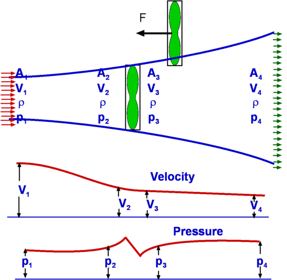 Figure 8: Analysis of a Wind Turbine A wind turbine (Fig 8) extracts energy from an air stream while a propeller adds energy to the air stream. The analysis follows the same lines. For the wind turbine the result is Power output is the rate of change in the kinetic energy of the stream, $$P_{output}=1/2m↖{.}(V_1^2-V_4^2)=1/2ρA_2V_2(V_1^2-V_4^2)$$Now the efficiency is given by the kinetic energy extracted divided by the total kinetic energy in the free stream for the given windwill area. Thus, Thus $$η_{optimum}={(V_4+V_1)(V_1^2-V_4^2)}/{2V_1^3}$$ $$η_{optimum}=1/2({1+V_4/V_1-(V_4/V_1)^2-(V_4/V_1)^3)$$ Maximum efficiency will occur when ${∂η_{optimum}}/{∂a}=0$ and will give a when $a=1/3$, .ie. $V_4/V_1=1/3$. At this point the maximum theoretical efficiency is 59.3%. Pressure Loss through a Sudden Expansion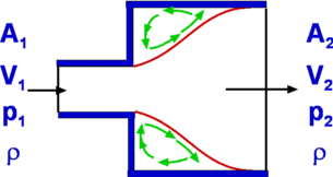 Figure 9 : Losses through a Sudden Expansion, Borda-Carnot Equation Consider a sudden expansion placed in a duct (Fig 9.). The flow does not follow the area changes as suddenly as the geometry does. Any flow will find the sudden area increase difficult to negotiate. In fact a recirculating flow develops as was seen in case of the orifice flow. This gives to losses which are reflected in the total pressure at downstream being reduced. It is possible to calculate this loss from a control volume analysis. Continuity EquationMomentum EquationThe forces upon the control volume sum up to Substituting in the momentum equation, i.e. substituting for V2 based on continuity gives, Bernoulli EquationDue to losses in energy it is not possible to connect stations (1) and (2) with the Bernoulli equation. However the total pressure relation at (1) and (2) can be used . Accordingly, $$P_{02}=P_2+1/2ρV_2^2$$ Total pressure loss is hence equal to substituting using the above formula for pressure difference, substituting for V2 based on continuity gives, $$P_{01}-P_{02}=ρV_1^2/2(1-2(A_1/A_2)+(A_1/A_2)^2)$$ $$P_{01}-P_{02}=ρV_1^2/2((A_1/A_2)-1)^2$$ Area ratio A1/A2 is less than 1.0, so static pressure after the expansion will be higher than the initial pressure. But based on the above formula there will always be a loss in total pressure; ie. loss in energy of flow. Measurement of AirspeedBernoulli equation readily allows the determination of the flow speed once the static and stagnation pressures are known. Rewriting the equation for Stagnation Pressure, It is therefore a matter of measuring the static and stagnation pressures at a given location. Static Pressure is conveniently measured by drilling a hole in the wall or the pipe, called the Pressure Tap (Fig. 10). A manometer or a pressure gauge is connected to the tap. During flow static pressure is communicated to the measuring device. Alternately one could use a Static Pressure probe shown in Fig. 11. This has surface holes in the tube which transmit the pressure to a measuring device.
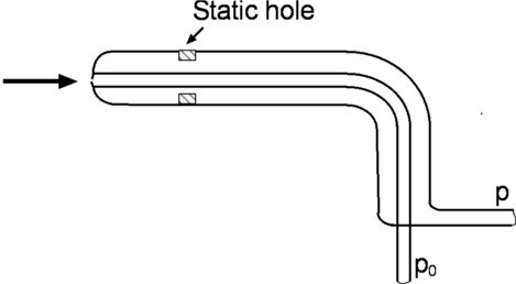
Measurement of stagnation pressure requires that the flow be brought to rest. A glass tube or a hypodermic needle aligned with the flow and facing upstream as shown in Fig. 12 will do the job. Alternately, what is called a Pitot Tube shown in Fig.13, with a hole facing upstream of the flow may be employed. The method shown in Fig. 14 allows both pressures to be measured at once. For an accurate determination of flow speed, static and stagnation pressures need to be measured simultaneously and in close proximity. This is made possible by a Pitot-Static tube shown in Fig. 15. This combines the static pressure probe and the pitot tube. The "static holes" and the "stagnation hole" are as near to each other as possible.
|