Fluid Mechanics

Elements of Potential Flow

Differential analysis of fluid motion is different from the analysis done in the previous section using control volumes. The focus now will be on a description of flow at any given point in the flow rather than on overall effects of the flow on a control volume. Point descriptions of flow are required to find the distribution of pressure on the surface of an aircraft wing or the distribution of velocities in a pipe for an air-conditioning system. This necessitates a more detailed knowledge of the flow field than that provided by the "integral approach" of the previous section.

The laws of conservation of mass, momentum and energy are applied to produce differential forms of the governing equations (and hence the name "differential approach". When all components are included, including viscosity, this leads to what are called the Navier-Stokes Equations. In situations where viscous effects make up only a small proportion of the flow then simpler solutions which are reasonably accurate can be employed. Only inviscid, incompressible flows will be considered in this section. The solution is then based only on the equation for mass conservation. This will allow the calculation of velocity components. Pressure is then obtained from Bernoulli equation.

The continuity equation will be derived. Then the concepts of stream function and velocity potential will be introduced. By analysing the kinematics of fluid motion, concepts of circulation and irrotationality can be demonstrated. Examples of simple flows such as a uniform flow, source and sink flow and vortex flow will be given. These flows can then be superimposed to produce solutions for more complex flows. Flow about a circular cylinder is analysed in some detail.

Conservation of Mass

The differential form of the equation for mass conservation can be found by considering a control volume at P(x,y,z) as shown in the figure below. The dimensions of the volume are dx, dy and dz and velocity components at point P will be u, v and w. Assuming that the mass flow rate is continuous across the volume we can calculate the mass flow rates at the various faces of the cell by a Taylor Series expansion. Accordingly,

$$\text"ML"=(ρu-{∂ρu}/{∂x}.{dx}/2).dy.dz\text"    ,    "\text"MR"=(ρu+{∂ρu}/{∂x}.{dx}/2).dy.dz$$
$$\text"MB"=(ρv-{∂ρv}/{∂y}.{dy}/2).dx.dz\text"    ,    "\text"MT"=(ρv+{∂ρv}/{∂y}.{dy}/2).dx.dz$$
$$\text"MA"=(ρw-{∂ρw}/{∂z}.{dz}/2).dx.dy\text"    ,    "\text"MF"=(ρw+{∂ρw}/{∂z}.{dz}/2).dx.dy$$

The net mass flow rate into the control volume as a consequence is given by,

leading to,

Applying the Reynolds transport theorem for mass will give,

thus

Cancelling out dx dy dz, we have,

This equation is known as the Continuity Equation. Note that it is a very general equation with hardly any assumption except that density and velocities vary continuously across the element.

Continuity Equation in Cylindrical Coordinates

The continuity equation was derived above using cartesian coordinates. It is possible to use this system for all flows, but sometimes the equations may become cumbersome. Many flows which involve rotation or radial motion are best described in cylindrical coordinates.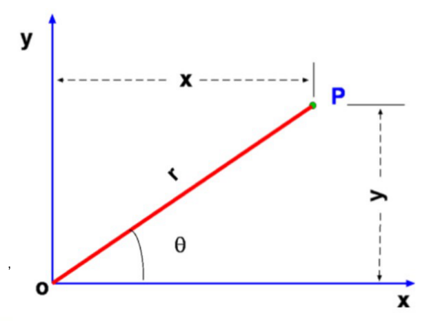

In this system, coordinates for point P are r,θ and z. The velocity components in these directions respectively are $v_r , v_θ \text"  and  " w$. Transforming between the cartesian and the cylindrical systems is provided by the relations,

The flow rates are given by,

As a consequence the continuity equation becomes,

Continuity Equation for steady flow

For a steady flow the time derivative vanishes. As a result continuity becomes

Continuity Equation for an Incompressible flow

For an incompressible flow density is a constant. Accordingly we have

As noticed for the control volume analysis the continuity equation for an incompressible flow is the same whether the flow is steady or unsteady.

Velocity Potential

Physically the driving force for fluid flow is pressure, however the introduction of a mathematical forcing function allows for a more standard equation and simpler solutions.

Velocity potential φ can be defined such that,

substituting these definitions into the continuity equation leads to the governing potential flow equation.

This is a standard version of the Laplace equation and many solutions are possible as will be seen later in this section.

Stream-function

Stream-function is amnother useful parameter for the study of fluid dynamics. It was arrived at by the French mathematician Joseph Louis Lagrange in 1781 and represents a physical quantity of the flow; volume or mass flow rate. It can be defined in both two and three dimensional flows. In three dimensional flow, stream function defines the surface of a stream tube but for simplicity, solutions here will be restricted to two-dimensional flows, where stream-function defines a stream line of the flow.

Consider a two-dimensional incompressible flow for which the continuity equation is given by,

Stream-function is a measure of volume flow rate between the streamlines of the flow, it is defined as a functional change at right angles to the flow direction, and as Velocity times Area is constant in incompressible flow, will predict the local velocities.

A stream function, ψ will satisfy the conditions,

Substituting these expressions into the continuity equation will give,

ψ, Stream-function is constant along a streamline

Consider a line given by $Ψ = C$, a constant, thus $dΨ=0$ and gives

after substituting for the gradients as velocities, -$v.dx+u.dy=0$

thus

Flow is thus always tangential to the streamlines and there will be no flow across a stream line.

Stream-function change (dψ) between two streamlines is proportional to the volumetric flow

Consider the volumetric flow through a small element of length (ds) placed between two streamlines as shown below. Flow the element must be the same as the addition of flow through the individual horizontal (dx) and vertical (dy) segments.

The volumetric flow through the element is given by

which indicates that the volumetric flow rate is proportional to the difference between stream functions. If we now integrate the between two stream lines ψ_A and ψ_B, then,

Stream Function in Polar Coordinates

The velocity components in polar coordinates are related to the stream function by,

Kinematics of Fluid Motion

A two-dimensional fluid particle, a square ABCD, can be tracked over time. It is subject to various forces and as a result undergoes a complex motion and a possible deformation as indicated. After a small time period it will assume a shape like A`B`C`D`.

This complex deformation of the element can be split into four basic constituents -

• Translation (movement of the centroid of the element)

• Linear Deformation (scaling of the size of the element)

• Rotation

• Angular Deformation (shearing of the element)

These deformations can be analysed separately to see their impact on the flow.

Translation

Translation is the type of motion where the element retains its shape. Its side do not undergo any change in length and the four angles do remain square. The square element ABCD, we have considered is bodily shifted from its position to a new one A`B`C`D`. If the motion is without acceleration in a steady, uniform flow it is easy to calculate the position of any particle in the fluid at different instants of time. But it should be noted that the fluid particles may undergo acceleration.

Considering now a particle in the fluid element we can write down an expression for its acceleration. At time t, the particle is at (x,y,z) and its velocity is given by,

where $V↖{→}$ is the fluid velocity. At time (t+dt) the particle will find itself at a different location and its velocity now is given by,

Consequently the change in velocity magnitude, $dV_p$ is given by,

The acceleration of the particle is obtained by dividing throughout by dt.

Now denoting the speed in x-direction, dx/dt by u, speed in y-direction dy/dt by v and speed in z-direction dz/dt by w, then

where dV_p/dt is the particle acceleration. The derivative dV_p/dt is usually denoted by DV/Dt and is called material derivative or the particle derivative or total derivative.

Linear Deformation

Considering the same element ABCD again. If the element has to undergo a linear deformation it is necessary that u velocity change in the x-direction and v velocity in the y-direction. Let the velocities at A be u and v. Then at B the x-direction velocity will be $u+{∂u}/{∂x}.dx$ and at D it will be $v+{∂v}/{∂y}.dy$. As a result the element stretches both in x and y directions and assumes a shape A`B`C`D`.

Now, the stretch in x-direction is given by distance BB' which is equal to

The corresponding change in the volume, $ʊ$, of the element (for a unit depth normal to the plane) is given by

Similarly the change in the volume of the element in the y-direction is given by,

Neglecting the small change in volume due to CC```C`C``, The total change in volume is

Thus the rate of change of volume expressed as a fraction of the initial volume is given by,

The left hand side is called the Volume Dilitation rate of the element. The right hand side of the equation is zero for all incompressible flows. Hence the volume dilitation rate for particles in potential flow will be zero.

Rotation

Considering the same element ABCD again, we notice that any rotation of AB or AD is brought about by a change in u velocity along y-direction and that of v velocity along x-direction. Let dα and dβ be the angles through which sides AB and AD rotate.

From the geometry, due to the rotation

Since angles dα and dβ are small we have,

Rotation or angular velocity of the element (about the z-axis) can be taken as the average of these two angular rates

Combining the above information,

Similarly, for rotation about the other axes,

In most cases the term vorticity is used and is defined as twice rotation rate, γ = 2 x ω

One group of flows has zero vorticity (i.e., rotation = 0 ). These are known as Irrotational Flows. For two dimensional, incompressible flows this is governed by the condition,

All potential flows are irrotational. This can be shown by substituting the gradient definitions for velocity into the above equation for vorticity.

It should be noted that the concept of Irrotationality applies to a fluid element in a given flow rather than to the flow itself. The main flow may contain a vortex where the streamlines are circles, but the individual elements of fluid may not rotate or distort making the flow irrotational. This is shown in the following figure where an irrotational flow about an aerofoil is shown.

Note that even though the streamlines follow a path which seems to curve and indicate an overall flow rotation, the particles themselves translate but do not rotate.

Angular deformation

If the particle is being sheared then the rate of shear strain for a two-dimensional flow this is given by the difference in rotation rate on each side.

Shear stress for the element can thus defined by

where μ is the viscosity of the fluid.

Circulation

Circulation is a measure of the total rotation induced by or contained in the flow field. Consider any closed curve C in the flow as shown below. Circulation is defined as the line integral around the curve of the arc length ds times the tangential component of velocity.

By applying Green's theorem circulation can be shown to be the sum of all vorticity within the area bounded by curve C,

Occurrence of Irrotational or Rotational Flows

The application of potential flow methods requires the flow to be irrotational. There are several cases where this can be applied and others where it cannot as the flow is rotational. A uniform flow is definitely irrotational, but this is a trivial flow and easy to predict. The region away from the surface of a solid body is also irrotational.

However new the surface this is not the case. A velocity gradient ${∂u}/{∂y}$ is set up when a fluid flows along the surface due the shear. The velocity right on the body surface is zero and it increases quickly normal the the surface away from the body. This region is highly rotational and is called the boundary layer. It is usually very thin and only effects a small region near the surface. Also due the flow separation and upper and lower surface boundary layer mixing the wake region will contain fluid shear and is also NOT irrotational.

It is worth noting that the flow is irrotational wherever the Bernoulli equation is valid.

Most external flows are likely to be inviscid flow and hence irrotational. This is broadly true until the speed becomes excessive and shock waves occur in the flow. The region just behind a shock in a high speed flow has severe gradients of velocity causing large shear and rotation.

Simple Examples of Plane Potential Flows

The examples considered here are such that there are analytical expressions for ψ, φ, u, and v. Hence they are exact solutions for the governing potential flow equations,

Potential Flow Equations in Cartesian Coordinates

The velocity components are given by,

The Laplacian is given by,

Equations in Polar Coordinates

Velocity Components:

The Laplacian is given by,

In the following images, the flow is defined by blue streamlines, having constant stream function value and green equi-potentials, having constant velocity potential value.

Uniform Flow

The simplest possible potential flow is a uniform flow, $V_{∞}$=constant

$$u=V_{∞}={∂φ}/{∂x}\text"    ,    "v={∂φ}/{∂y}=0$$

On integration,

where C is the constant of integration, which can be chosen arbitrarily. In most cases C=0 can safely be set. This will put the ψ = 0 streamline through the origin (0,0) of the flow field.

The stream function for uniform flow can be easily calculated in a similar manner, and is given by,

It is also possible to define velocity potential and stream function for uniform flows which incorporate angle of attack such that,

Source or Sink

Considering a radial flow going away from the origin with a velocity, v_r as shown below. This constitutes a Source Flow. This is a purely radial flow with no component of velocity in the tangential direction, i.e. $v_θ=0$.

If m is the volumetric flow rate then, $m=2πr v_r$

or

Velocity potential and stream function for this flow :

It is easily verified that tangential velocity ($v_θ$) is zero for this flow. The conservation of mass equation for the source flow means that the Volumetric flow rate (mass flow rate divided by density) is constant in a radial direction and is equal to m, which is called the strength of the source.

Note that the radial velocity v_r becomes infinite at r = 0. So the origin is a singularity of this flow. If m is negative we have a flow which moves inward to the origin and is called a Sink flow. This again has a singularity at the origin.

Vortex

Another primary flow is one where radial velocity is zero and only flow in a circumferential direction occurs. This is Vortex flow.

The velocity potential and stream function are given by,

The velocity components are given by

It is seen that $V_θ$ is infinite at the origin and decreases as r increases and becomes zero as r approaches infinity.

Is this a contradiction? How is it that a vortex flow is irrotational? Note that the term "Irrotational" refers to the behaviour of a fluid element and not to the path taken by it. At an elemental level the flow is still irrotational. Such a vortex is called a Free Vortex. A familiar example is that of a bath tub vortex.

In contrast to this is Solid Body rotation. This has a velocity given by $v_θ=Kr$, with a zero velocity at the origin. The velocity increases as one moves away from the origin. A cup of tea that is being continually stirred is a good example.

It can be shown that the velocity potential for a solid body rotation is not uniquely defined and that such a forced flow is not a valid potential flow. A solid body rotation is not an irrotational flow.

Circulation around a Vortex

The circulation due to a vortex can be calculated as follows,

which is non-zero for our irrotational flow. As there is a singularity in our region, namely at, r = 0, the integral is non zero. If we exclude the singularity by taking a path that does not include this region then the circulation around that path is zero. Clearly the irrotational vortex flow is induced by an extremely strong forced rotation centered on an extremely small point at the origin.

It is usual to write the equation for velocity potential and stream function in terms of circulation Γ, thus

Note that for a positive value of circulation, the vortex flow is induced in an anti-clockwise direction.

A Source-Sink Pair

Considering a source and a sink placed at (-a,0) and (a,0) respectively. A property of the governing potential flow equation is that the superposition of a valid flow with another valid flow produces a third valid flow. So by adding the separate streamfunctions for the source and the sink we have a streamfunction for the combination given by,

By taking tangents of the two sides (after manipulation),

From the geometry it follows that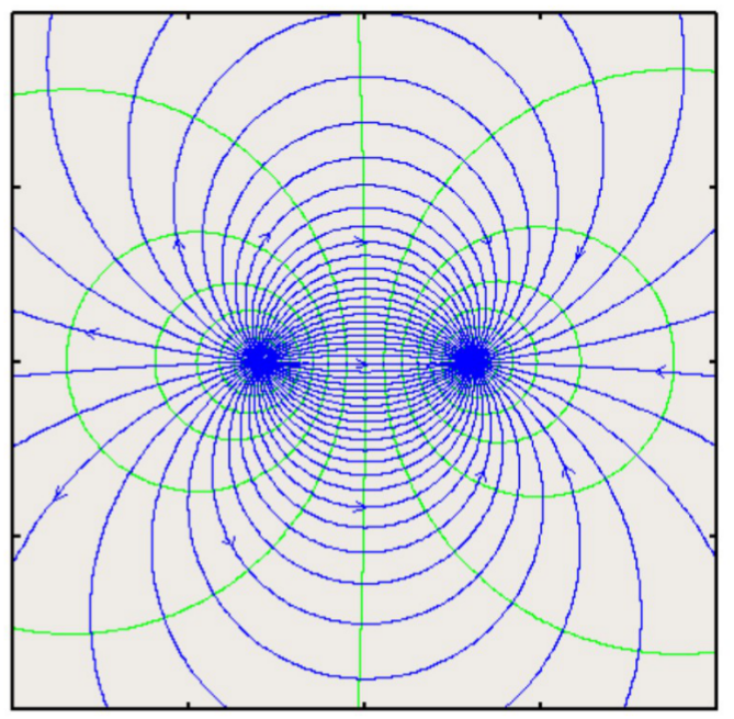

Upon substituting,

so that

When the distance between the source and the sink becomes smaller, i.e., when (a) is small we have,

Doublet

A Doublet is formed when the source and sink approach each other, i.e. $a→0$ and at the same time $m→∞$ such that ${ma} /π$ is constant, so that

As a consequence the stream function becomes

The velocity potential is

Potential lines for a doublet are sketched above. It is seen that the streamlines are circles which are tangential to the x-axis while the equipotential lines are also circles but tangential to y-axis.

Superposition of Elementary Flows

Simple flows such as uniform flow, source flow, vortex and doublet flow serve as primary components of potential flow. By combining these flows it is possiblt to build up more complicated flows.

All flows discussed are linear. As the governing continuity equation is linear then if $A$ and $B$ are two solutions, then $mA±nB$ (where $m$ and $n$ are scale factors) is also a solution.

The following programs canbe used to create streamlines and velocity potential lines for various cases of potential flow element superposition.

• streamf.exe -- Potential Flow stream line plotting program. (MS windows executable)
• velpot.exe -- Potential Flow velocity potential plotting program. (MS windows executable)
• Potential Flow Arbitrary Stream Function plotting program.

Uniform Flow and a Source

If a source is placed in the path of a uniform flow then the following flow is produced. The stream function and the velocity potential for the resulting flow are given by adding the two stream functions and velocity potentials as follows,

One of the interesting features to determine for the resulting flow is the creation of a stagnation point, i.e., point where the velocity goes to zero.

It is clear that for this flow the stagnation point will occur on the x-axis. The location can be arrived at purely intuitively. The source produces a radial flow of magnitude

while the uniform flow produces a velocity of $V_∞$ in the positive x-direction. Where these two cancel out will be a stagnation point. A negative radial flow that can cancel the uniform flow is possible only to the left of the x-axis, say at x = -b. Hence, at this point,

leading to

At x = -b, θ = π and r = b. Substituting these values in the expression for ψ, this the value at the stagnation point will be

The equation for the streamline passing through the stagnation point is obtained as follows,

thus

$$r/b\sin(θ)+θ=π\text"    or    "y=b(π-θ)$$

The streamlines for this flow are shown in the above figure. The red stream line is the boundary between the two flow components and as the properties of a streamline are such that there is no flow across the line, then the red streamline could be treated as the boundary of a solid surface. In the present example, if we ignore the streamlines inside the "body" we have described the flow about a solid body. This body is referred to as a Rankine Half Body as it is "open" at the right hand end.

Limits of θ for this body are 0 to 2π. At these values we have y approaching $±πb$, which is called the half width of the body.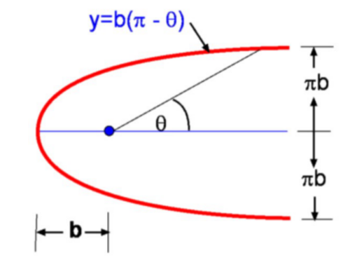

The velocity components for this flow are given by

If the pressure in the free stream is $P_∞$, it follows from Bernoulli Equation that along a streamline around the body,

thus allowing pressure to be calculated on the surface of the object. Usually in aerodynamic applications involving significant velocities and pressures any contribution due to elevation changes is negligible. The equation for pressure assumes a simple form,

It is also possible to calculate the maximum velocity over the surface of the body. This occurs at the location $θ=63^{o}$ and is approximately equal to $1.26V_∞$.

Rankine Oval

In the previous example, a half body open at one end was constructed. A closed body can be created by adding a trailing sink which will capture the mass flow from the source and thus close the rear of the shape. The stream function for this source/sink pair in a stream is given by

or in cartesian coordinates,

When the streamlines for this flow are plotted (see below) one discovers that the ψ = 0 stream (shown in red) forms a closed curve. This forms the solid body or boundary of an oval. Shapes such as this are called Rankine Ovals.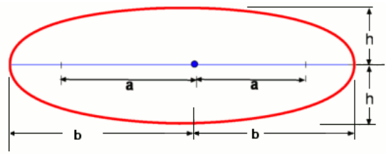

The distance to the stagnation points from the origin or the Half Body Length is given by

The other feature of interest, Half Width is found by determining the point of intersection of y-axis with the body, i.e.,ψ = 0 line. An expression for h is,

The solution for this non-linear equation is to be obtained by iteration.

Rankine ovals include a wide range of bodies which can be obtained by varying the value of the parameter ${πV_∞a}/m$. 1These could be bodies stretched in any of the two directions. When stretched in x-direction one obtains elliptic bodies with a small half width compared to the span. The solution obtained could be a good approximation to the flow especially if viscous effects are small. On the other hand a considerable half width would indicate a bluff body prone to effects like separation. The solution obtained can hardly be accepted in this case.

Flow Around a Circular Cylinder

Flow around a circular cylinder can be produced from the previous example by bringing the source and the sink closer together. In the limit this produces a uniform flow in combination with a doublet.

The stream function and the velocity potential for this flow are given by,

$$ψ=V_∞r\sin(θ)-{K\sin(θ)}/r\text"    ,    "φ=V_∞r\cos(θ)+{K\cos(θ)}/r$$

The velocity components are given by,

$$v_r=1/r{∂ψ}/{∂θ}=\cos(θ)(V_∞-K/r^2)$$
$$v_θ=-{∂ψ}/{∂r}=-\sin(θ)(V_∞+ K/r^2)$$

The radial velocity is zero when,

This condition will identify the surface of the cylinder. Thus the radius of the cylinder (a) is given by,

The equations for the streamline, velocity potential and the velocity components can be re-written in terms of the size (radius = a) of the cylinder.

The velocity components on the surface of the cylinder are obtained by putting r = a in the above expressions. Accordingly,

The stagnation point on the cylinder will this be at θ = 0 and 180⁰ and a maximum velocity will occur at θ = 90⁰ and 270⁰. Note: the sign of the $v_θ$ component is negative because of the definition of surface directions and polar axes. The actual surface velocity at these maximum points will have a magnitude of $2V_∞$ and be in the same direction as the free stream flow.

The surface pressure distribution is calculated from Bernoulli equation,

$$P_∞=1/2ρV_∞^2=P+1/2ρV^2$$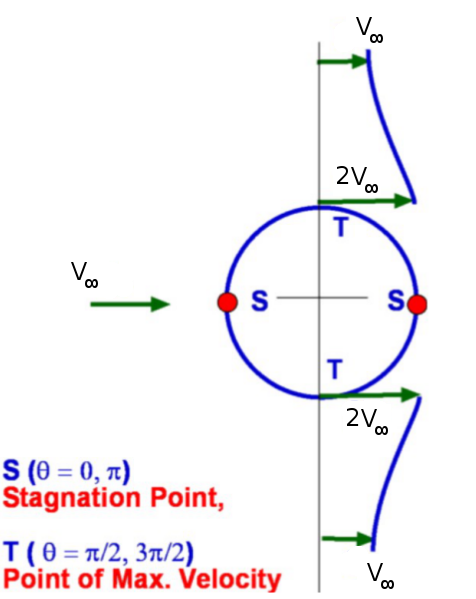

Substituting for surface velocity gives,

We can also express pressure in terms of pressure coefficient, C_p,

which gives,

A symmetry about y-axis is apparent. When compared to the experimentally observed Cp distribution, there is some agreement in the region between θ = 0⁰ and 90^0.. The deviation from there to the rear of the cylinder is because this region is dominated viscous forces giving rise to separation. The pressure tends to remain constant in the separated region and this has an effect upstream. For High Re, a turbulent attached layer is present up to approximately 130^o, but for low Re number laminar boundary separation occurs at 90^o and the pressure field is different from the ideal.

Symmetry in the theoretical C_p distribution about both y-axis and x-axis shows that drag and lift forces about the cylinder are each zero. In contrast experimental results show a significant drag component due to the separation which produces a large area of low pressure behind the cylinder.

Symmetric pressure loading for a non-rotating cylinder.

Flow about a Lifting Cylinder

A lifting flow can be generated by adding a vortex to the flow about a cylinder just described. The assumed positive direction for rotation is clockwise so take care when looking at the sign of induced velocity components. The stream function and the velocity potential now become,

$$ψ=V_∞r\sin(θ)(1-a^2/r^2)+Γ/{2π}\ln(r)$$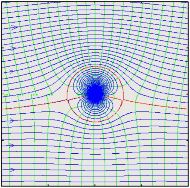
$$φ=V_∞r\cos(θ)(1+a^2/r^2)-Γ/{2π}θ$$

Consequently the velocity components will be,

At r = a, the radial velocity is still zero so that this is still the equivalent to a surfce of a body. The tangential velocity on the surface of the cylinder is given by,

The stagnation points for this flow will be found by calculating locations where surface velocity is zero.

$$\sin(β)=Γ/{4πV_∞a}$$

The surface velocity can now be written as

Stagnation Points for a lifting circular cylinder

The stagnation points shown above are for the case when there is circulation imposed on the cylinder is small was such that $Γ<4πV_∞a$. However for larger values of circulation the angle β, hence the position of the stagnation points will reach a limit of 90^o. This will occur when $Γ=4πV_∞a$. If the rotation is further increased the stagnation point will no longer be found on the cylinder surface, but will move down into the flow and fluid will be entrained with the rotating cylinder (d) as shown below.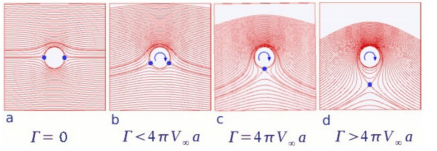

Surface Pressure Distribution and Lift

The surface pressure is calculated from the Bernoulli equation as

or

$$C_P=1-({v_{θ(surface)}/V_∞)^2=1-4(\sin(θ)+\sin(β))^2$$

The C_p distribution is plotted above. Asymmetry about x-axis is evident indicating the generation of lift. A small amount of rotation will cause a large pressure imbalance between upper and lower surface and hence a large lift. Fore and aft pressure is still maintained as there is no separation in ideal flow so Drag is still zero.

The magnitude of the lift force, L, is calculated by integration as

The components from stream static pressure and velocity will be balanced around the cylinder and their integration will be zero.

Integration of the $\sin^2(β)\sin(θ);$ term and the $\sin^3(θ)$ from $0→2π$ also results in zero.

when substituing for the expression relating $\sin(β)$ and $Γ$

Magnus Effect

A force is produced when circulation is imposed upon a cylinder placed in uniform flow. This force is the lift. This effect is called Magnus Effect in honour of the scholar Heinrich Magnus (1802 - 1870). It also works to a lesser extent on spheres so sports involving balls, such as golf, baseball, tennis see this effect in action. A spinning ball when hit in a horizontal direction follows a curved trajectory because of this effect.

Kutta-Joukowsky Theorem

The result derived above, namely, $\text"Lift"=ρV_∞Γ$ is a very general one and is valid for any closed body placed in a uniform stream that is creating circulation. It is named the Kutta-Joukowsky theorem in honour of Kutta and Joukowsky who proved it independently in 1902 and 1906 respectively.

The theorem finds considerable application in calculating lift around aerofoils and will be used extensively in later sections covering aerofoil and wing analysis.