Fluid MechanicsProperties of Fluids Fluid Statics Control Volume Analysis, Integral Methods Applications of Integral Methods Potential Flow Theory Examples of Potential Flow Dimensional Analysis Introduction to Boundary Layers Viscous Flow in Pipes |
Viscous Flow in PipesPipes are closely associated with fluid flow. Many examples of pipe flow are encounted in every-day life - for water and gas supply at houses and offices, in fluid machinery, for transporting oil over long distances, etc. A flow can be an Internal flow or an External Flow. Internal flows are further classified into Pipe Flows and Open Channel Flows. A pipe flow is one where the fluid fills the conduit completely. The main driving force is pressure although gravity may also be contributing to the flow. Open Channel Flow is open where the fluid does not fill the conduit completely. The driving force is gravity. 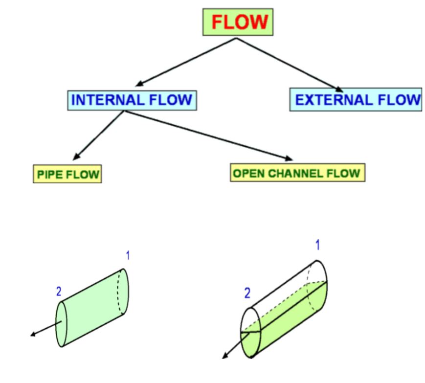 Figure 1: Flow Classification Classification of Flows, Laminar and Turbulent FlowsA flow can be Laminar, Turbulent or Transitional in nature. Very different results are obtained depending on which type of flow is encountered. This was demonstrated in the experiments conducted by Osborne Reynolds (1842 - 1912). Into a flow through a glass tube (Fig.2.) he injected a dye to observe the nature of flow. When the speeds were small the flow followed a straight line path (with a slight blurring due to dye diffusion). As the flow speed was increased the dye fluctuated and intermittent bursts were observed. As the flow speed was further increased the dye was blurred and began to fill the entire width of the pipe. These different results demonstrate Laminar, Transitional and Turbulent Flows. 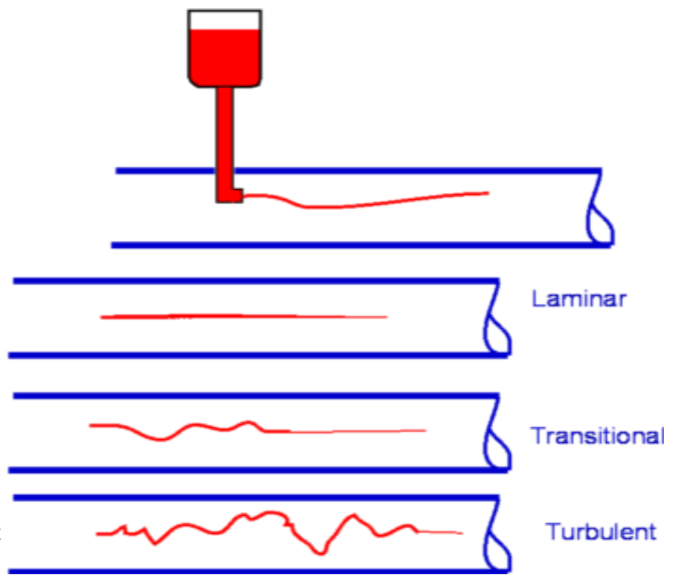 Figure 2: Reynolds Experiment To measure in detail what is happening an experiment may be conducted using modern day electronic equipement, Hot Wire Anemometer. This instrument measures instantaneous velocities at a point. The traces of velocity at the three regimes of flow are shown in Fig.3. Laminar flow has a predominant velocity in the main flow direction, turbulent flow has a significant component of velocity in the flow normal direction. While laminar flow is "orderly" turbulent flow is "Random" and "Chaotic". 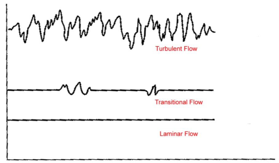 Figure 3: Hot Wire Signals for Turbulent flow (top), Transitional flow (middle) and Laminar Flow (bottom) Flow in a pipe is laminar if the Reynolds Number (based on diameter of the pipe) is less than 2100 and is turbulent if it is greater than 4000. Transitional Flow prevails between these two limits. However these are generalised results and some experiments have found preserved laminar flow at very high Reynolds number through carefully monitored conditions or turbulent flow at lower Reynolds numbers with very rough surfaces. 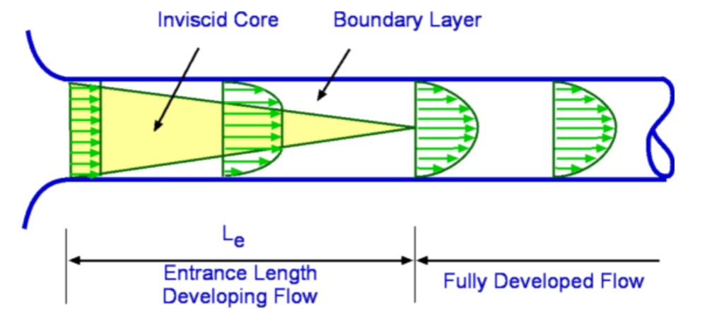 Figure 4: Flow at the entrance to a pipe Consider a flow entering a pipe. The entering flow is assumed to be uniform, so inviscid. As soon as the flow encounters the walls of the pipe velocity changes take place. Viscosity imposes a "No Slip" condition at the wall of the pipe. Consequently the velocity components are each zero on the wall, ie., u = v = 0. The flow adjacent to the wall decelerates as it travels along the pipe. The boundary layer close to the wall has an established velocity profiler. Viscous effects are dominant within the boundary layer. Outside of this layer the inviscid core remains until boundary growth from opposite sides joins at the centerline. This can be seen in Fig.4. Once this has taken place, the inviscid core terminates and the flow is completely viscous. The flow is now called a Fully Developed Flow. The velocity profile becomes parabolic and does not vary in the flow direction. In this region the pressure gradient and the shear stress in the flow are in balance. The length of the pipe between the start and the point where the fully developed flow begins is called the Entrance Length. Denoted by Le, the entrance length is a function of the Reynolds Number of the flow. In general,
$$L_e/D≈0.06({Re}_D)\text" , for a Laminar Flow"$$ where ReD is Reynolds number based on "Entrance Diameter". At critical condition, i.e., ReD =2300, the Le/D for a laminar flow is 138. Under turbulent conditions it ranges from 18 (at ReD = 4000) to 95 (at ReD=108) Pressure along the pipeThe forces acting along the pipe are inertial, viscous force due to shear and the pressure forces. Gravity can be ignored if the pipe is horizontal. When the flow is fully developed the pressure gradient and shear forces balance each other and the flow continues with a constant velocity profile. The pressure gradient remains constant. In the entrance region the fluid is decelerating. A balance is achieved with inertia, pressure and shear forces. The pressure gradient is not constant in this part of the flow and decreases as shown in Fig.5 . 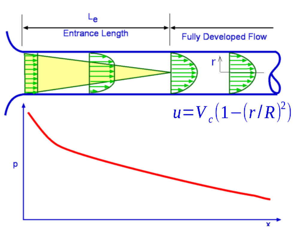 Figure 5 : Pressure distribution along the flow in a pipe. Fully Developed Laminar Flow in a PipeConsidering a fully developed laminar flow in a pipe it is possible to derive an expression for the velocity profile and then calculate useful practical results. This derivation can be carried out in a number of ways - (1) by a Control Volume Analysis, (2) from Navier-Stokes Equation or (3) by Dimensional Analysis. Volumetric Flow RateA quantity of interest in pipe flows is the volumetric flow rate, which is obtained by integrating the velocity profile. Considering a disc of thickness dr at a radius r then $$dQ=(2πr.dr)u$$ integrating $$Q=∫_0^R 2πV_c(1-(r/R)^2)r.dr$$ leading to $$Q={πR^2V_c}/2$$ If an average velocity, V, is defined such that $V=Q/A$ it can be verified that $$V=V_c/2={ΔPD^2}/{32μl}$$ The volumetric flow rate written in terms of pressure gradient becomes, $$Q={πD^4ΔP}/{128μl}$$ Correction for non-horizontal pipesIf the pipe considered in the previous analysis was not horizontal, then gravity effects should be included when calculating velocity and volumetric flow rates. Referring to Fig.8, if the flow is inclined at an angle θ to the horizontal, the pressure difference term needs to be modified. 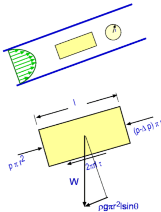 Figure 8: Flow through an inclined pipe. Accordingly, the force balance becomes $${ΔP-γl\sin(θ)}/l=2τ/r$$ The pressure difference term in other equations needs to be replaced as well. Accordingly, $$Q={πD^4(ΔP-γl\sin(θ))}/{128μl}$$ and $$V={(ΔP-γl\sin(θ))D^2}/{32μl}$$ Energy Considerations, Friction factor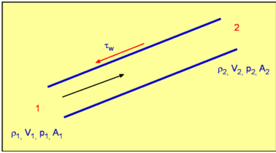 Figure 9: Energy balance for a pipe flow. Again considering the pipe flow as in the previous section, an energy analysis can be carried out. With reference to Fig. 9, for a mass balance, $$ρ_1A_1V_1=ρ_2A_2V_2$$ Since the flow is incompressible and the pipe cross-section area is constant, $$V_1≈V_2=V$$ Now applying the energy equation for a steady flow, $$(P/γ+αV^2/{2g}+z)_1=(P/γ+αV^2/{2g}+z)_2+h_f$$ Note that every term in the above equation has the dimension of length. As a fully developed flow is being considered , then α1 = α2 . There are no external features between (1) and (2) which could add or remove energy. As a result, loss of head is given by, $$h_f=(P_1/γ-P_2/γ)+(z_2-z_1)$$ A force balance in the x-direction on a control volume gives, $$ΔPπR^2+γπR^2L\sin(θ)-τ_w2πRL=0$$ Note that, $L\sin(θ)=z_2-z_1=Δz$ $$ΔPπR^2+γπR^2Δz-τ_w2πRL = 0$$ Dividing by $πγR^2$ gives, $${ΔP}/γ+Δz={2τ_wL}/{γR}$$ An inspection of these equations shows that $$h_f={2τ_wL}/{γR}\text" or "h_f={4τ_wL}/{γD}$$ Again this result is valid for both laminar and turbulent flows. Dimensional AnalysisThrough a dimensional analysis it is possible to derive an expression for "loss of head" in a pipe flow. Assuming that pressure drop is proportional to pipe length it can be shown that $${ΔP}/{1/2ρV^2}={32μlV}/{1/2ρV^2D^2}={64}/{Re}l/D$$ Thus pressure drop now becomes, $$ΔP=fl/D{ρV^2}/2$$ with $$f={{ΔP}(D/l)}/{1/2ρV^2}$$ The non-dimensional quantity fis referred to as "Darcy's Friction Factor". For a laminar flow it is given by $f={64}/{Re}$ . It is possible to show that $$f={8τ_w}/{ρV^2}$$ Turbulent Flow through PipesTurbulent Flows can be calculated using the Navier-Stokes equation along with a model for turbulence. Several models have been developed for the purpose. They start from the simple algebraic models to the most involved Reynolds stress modelling. In addition, Direct Numerical Simulation (DNS) and Large Eddy Simulation (LES) are among the recent computational methods to handle turbulent flows. A full discussion of these numerical methods is beyond the scope of this section on Fluid Mechanics. Based on experimental findings a velocity profile can be arrived at called the Logarithmic Overlap Law. This is constructed as shown below. Logarithmic Overlap Law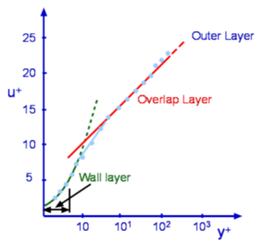 Figure 10 : Logarithmic Overlap Law 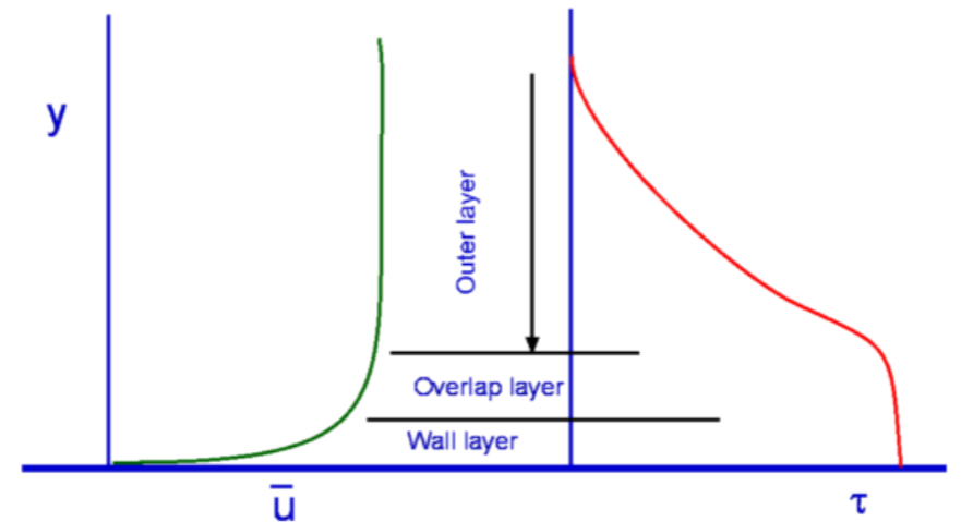 Figure 11 : Velocity and Shear Stress profiles for a Turbulent Boundary Layer A typical boundary layer velocity profile for a turbulent flow about a flat plate is shown in Fig.10. This profile is studied inconjunction with the shear stress profile also shown in Fig. 11. The profile is marked by three distinct zones or layers- (1) Wall Layer, (2) Outer Layer and (3) Overlap Layer. Wall LayerThe wall layer is the one closest to the wall. In this layer the flow is dominated by viscous shear force. From Fig. 11, it is clear that shear stress is almost constant in this layer. By defining a friction velocity as $$u^{*}=√{τ_w/ρ}$$ It is established that for this layer, $$u^{+}=y^{+}$$ where $$u^{+}={u↖{-}/u^{*}\text" and "y^{+}={u^{*}y}/ν$$ Since, by definition, $ν=μ/ρ$, the wall layer extends from the wall to a y+ of about 5 and merges with the logarithmic profile in the Overlap region at around a y+ of 30. Overlap LayerOverlap layer is in between the wall layer and the outer layer. As the name indicates, both laminar and turbulent shear stresses prevail in this region. The velocity profile is given by the logarithmic law, $$u^{+}=1/κ\ln(y^{+})+B$$ where the Karman constant, κ is 0.41 and B≈5.0. Outer LayerOuter Layer is next to the Overlap Layer. It is found that in this layer u is independent of μ , molecular viscosity. The flow is dominated by turbulent shear. The velocity profile is now given by the Velocity Defect Law. $${U-u↖{-}}/u^{*}=G(y/δ)$$ Power Law Velocity ProfileIn many engineering calculations, it is possible to simplify this complex velocity profile model by using a simple power law approximation, $${u↖{-}}/U=(y/R)^{1/n}=(1-r/R)^{1/n}$$ The exponent "n" is a function of Reynolds Number. However, n=7 is a good approximation for a wide range of pipe flows and is the one commonly used. It is referred to as the "One seventh power law". This power law cannot however be used to calculate the wall shear stress as it gives an infinite velocity gradient at the wall. For a power law it can be shown that the ratio of average velocity to the centreline velocity is given by, $${V_{avg}}/U={2n^2}/{(n+1)(2n+1)}$$ |