Fluid MechanicsProperties of Fluids Fluid Statics Control Volume Analysis, Integral Methods Applications of Integral Methods Potential Flow Theory Examples of Potential Flow Dimensional Analysis Introduction to Boundary Layers Viscous Flow in Pipes |
Introducton to Boundary LayersViscous Effects in External FlowsIn previous sections viscosity was neglected in most of the analyses. The potential flows that were considered in the previous sections are inviscid, i.e., ignored viscosity. In reality these flows are purely theoretical. In the case of flow about a cylinder viscosity will alter the flow completely in the aft of the cylinder. Any real flow in nature incorporates viscosity. It is viscosity that gives rise to many of the interesting physical features of a flow. The layer of flow near to a surface is dominated by viscosity. This layer is called a boundary layer and will be the focus of this section. Boundary layer growth, transition between smooth and turbulent flow, changes due to pressure gradient and boundary layer separation will be covered in this section. Boundary Layer FlowFor flow over a plate, right a the surface a "No Slip" condition occurs. This means that that the fluid is stuck to the surfce and does not move relative to the surface. This is a typical effect of viscosity. 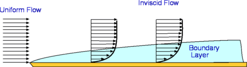 Figure 1: Formation of a Boundary Layer In Fig 1 a uniform flow in front of a flat plate at a speed $U_∞$ is considered. Where the flow touchs the plate, the no slip conditions occurs. As a result, the velocity on the surface of the body becomes zero. Since the effect of viscosity is to resist fluid motion, the velocity will be slowed by the action of the zero velocity flow at the surface. This action is reduced at distances which are further from the plate until the speed is again equal to the freestream value of $U_∞$. A velocity gradient is set up in the fluid in a direction normal to flow. Thus a layer establishes itself close to the wall. This is called the Boundary Layer. The boundary layer is not a static phenomenon. It is dynamic. The thickness of boundary layer (the height from the solid surface where the flow is again 99% of free stream speed) continuously increases downstream along the plate. A shear stress develops on the solid surface. It is this shear stress that causes drag on the plate. The Boundary Layer has a pronounced effect upon any object which is immersed and moving in a fluid. Drag on an aircraft or a ship and friction in a pipe are some of the common manifestations of boundary layer. Understandably, boundary layer analysis has become a very important branch of fluid dynamic research. Laminar and Turbulent Boundary LayersA boundary layer may be laminar or turbulent. A laminar boundary layer is one where the flow is smooth and layered, i.e., each layer slides past the adjacent layers. This is in contrast to a turbulent boundary layer as shown in Fig. 2 where there is mixing between the layers. In a laminar boundary layer any exchange of mass or momentum takes place only between adjacent layers on a microscopic scale which is not visible to the eye. Consequently molecular viscosity μ is able predict the shear stresses produced. Laminar boundary layers are found only when the Reynolds numbers are small. 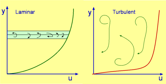 Figure 2 : Typical velocity profiles for laminar and turbulent boundary layers A turbulent boundary layer on the other hand is marked by random mixing of fluid across several layers. The mixing is on a macroscopic scale. Packets of fluid may be seen moving up and down with the layer. Thus there is an exchange of mass, momentum and energy on a much bigger scale compared to a laminar boundary layer. A turbulent boundary layer forms at larger Reynolds numbers. The scale of mixing cannot be handled by molecular viscosity alone. Calculation of turbulent flow relies on a convection parameter called Turbulence Viscosity or Eddy Viscosity. There is no exact expression for this and it needs to be numerically modelled in all cases. Several models have been developed for the purpose of simplifying this statistically varying flow. 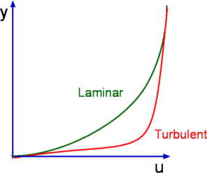 Figure 3 : Typical velocity profiles for laminar and turbulent boundary layers The turbulent layer can be described using an average velocity profile. As a consequence of intense mixing, a turbulent boundary layer has a steep gradient of velocity at the wall and therefore a large shear stress. In addition heat transfer rates are high. Typical laminar and turbulent boundary layer profiles are shown in Fig 3. Based on these approximate velocity profiles the growth rate of the boundary can be caluclated. Grow rate represents the rate at which the boundary layer thickness, δ increases along the late. Growth rate of a laminar boundary layer is small. For a flat plate it is given by $$δ/x={5.0}/√{{Re}_x}$$ where Rex is the Reynolds Number based on the distance from the front of the plate. For a turbulent flow it is given by $$δ/x={0.385}/{{Re}_x^{0.2}}$$ Wall shear stress is another important parameter for boundary layers. It is usually expressed as Skin Friction Coefficient and defined as $$C_f=τ_w/{1/2ρU_∞^2}$$ where $τ_w$ is the wall shear stress given by $$τ_w=μ({∂u}/{∂y})_{y=0}$$ and $U_∞$ is the free stream speed. Skin friction for laminar and turbulent flows are
$$C_f={0.664}/√{{Re}_x}\text" -Laminar Flow"$$ Separation of FlowPressure gradient is another of the factors that influences the growth of the boundary layer flow. The shear stress caused by viscosity has a retarding effect upon the flow. This effect can however be overcome if there is a negative pressure gradient applied to the flow. A negative pressure gradient is termed a Favourable pressure gradient and represents the case where flow velocity outside the boundary layer is accelerating. A positive pressure gradient has the opposite effect and is termed an Adverse Pressure Gradient. In this case the external flow is decelerating. Fluid finds it difficult to negotiate an adverse pressure gradient. The growth rate of the boundary is increased significantly by an adverse pressure gradient. 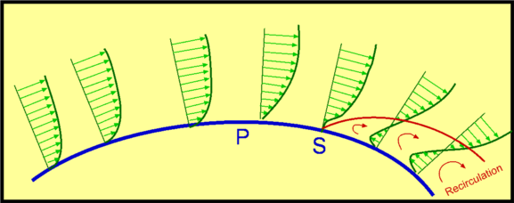 Figure 4 : Separation of flow over a curved surface One of the severe effects of an adverse pressure gradient is to separate the flow away from the body surface. For the flow past a curved surface as shown in Fig. 4 profiles are shown for an adverse pressure gradient caused by the shape of the surface. The geometry of the surface is such that a favourable gradient in pressure to start with and up to a point P. The negative pressure gradient will counteract the retarding effect of the shear stress in the boundary layer. There is then an adverse pressure gradient downstream of P. The adverse pressure gradient begins to retard the flow. This effect is felt more strongly in the regions close to the wall where the momentum is lower than in the regions near the free stream. As indicated in the figure, the velocity near the wall reduces and the boundary layer thickens. A continuous retardation of flow brings the wall shear stress at the point S on the wall to zero. Here the flow in the vicinity of the wall is completely stopped, not just the surface no slip flow. From this point onwards the shear stress becomes negative and the flow reverses and a region of recirculating flow develops. The flow no longer follows the contour of the body. The flow has separated. The point S where the shear stress is zero is called the Point of Separation. Depending on the flow conditions the recirculating flow may terminate and then the flow may reattach to the body. A separation bubble is formed. There are a variety of factors that could influence this reattachment. The pressure gradient may become favourable due to further changes in body geometry. The other factor is that the flow which was initially laminar may undergo transition within the bubble and may become turbulent. A turbulent flow produces more energy and momentum in the near wall region. This can remove the recirculating flow region and the flow may reattach. 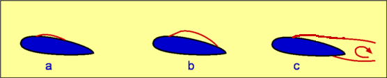 Figure 5 : Separation bubble over an aerofoil On aerofoils at low angles the separation may occur near the leading edge and give rise to a short bubble by transition to turbulence. At high angles the separated flow may not reattach and simply merge with the wake region. This will result in stall of the aerofoil (loss of lift, increase in drag). DragDrag is the force that opposes motion. An aircraft flying has to overcome the drag force upon it, a ball in flight, a sailing ship and an automobile at high speed are some of the other examples. It is clear that viscosity is the agent that causes drag. It gives rise to boundary layers on solid surfaces. The is shear stress in boundary layer applies a retarding force to the body . This is shown for an aerofoil surface in Fig 6. and is termed Skin friction Drag. 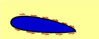 Figure 6 : Shear stress on a body There is another mechanism that can cause drag. This is the pressure difference upon the flow. It can come about due to geometric effects and due to separation. This is called Pressure Drag or Form Drag, since it is due to the body geometry. The sum of pressure drag and skin friction drag constitutes Drag about the body or Profile Drag. 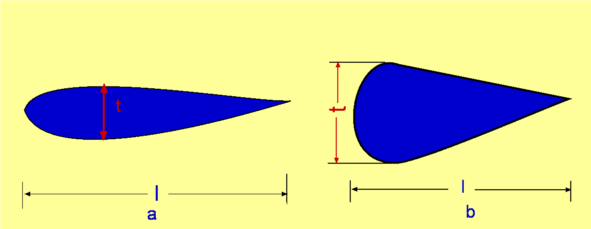 Figure 7 : Effect of thickness of body on drag The shape of the body determines the relative magnitude of the drag components. A thin body (small t/l ratio) as shown in Fig. 7 obviously causes less pressure drag. Almost all drag comes from skin friction. A thick body (large t/l ratio) is readily prone to separation and produces considerable pressure drag. Streamlining a body to avoid separation will decrease pressure drag considerably. A bluff body like a cylinder or a sphere or a flat plate placed normal to flow will cause separation and lead to pressure drag will be far greater than the skin friction drag. In case of a flat plate placed parallel to flow (Fig. 8 ), it is the skin friction drag that dominates. On the other hand, in case of a flat plate placed normal to flow, it is the pressure drag that dominates. In the latter case, the plate behaves like a blunt body with separation at the corners leaving a low presure region at the rear which contributes to drag. 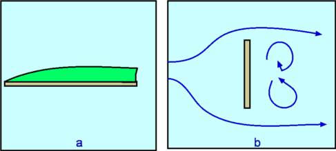 Figure 8 : Drag about a flat plate Drag CoefficientDrag force is non-dimensionalised as $$C_D={\text"Drag"}/{1/2ρ_∞U_∞^2A}$$ where CD is defined as Drag Coefficient. $U_∞$ is the free stream speed, $ρ_∞$ is the free stream density, A is the area. The area to be used in this calculation depends upon the application. In case of a cylinder it is the projected area normal to flow. For a flow past a thin flat plate, it will be the surface area of plate exposed to flow. The relative importance of the two kinds of drag is very apparent in case of flow over a circular cylinder or a sphere. The flow depends strongly upon Reynolds number as is shown in Fig. 9. When the Reynolds number is small (1 or below) the flow behaves like a potential flow. There is no separation. The drag is all due to skin friction. As the Reynolds number is increased this drag decreases. At Reynolds numbers around 2 - 30, there is a separation of boundary layer, but the wake is of a limited length. The eddies formed are fixed behind the cylinder. For Reynolds numbers around 40 - 70, there is a periodic oscillation of the wake. For higher Reynolds numbers the eddies break off from the cylinder. As the Reynolds number is increased, the eddies are continuously shed from the cylinder and washed downstream. Two rows of vortices are formed called the Vortex Street. Now the pressure drag contributes to almost 90% of the total drag. The value of CD reaches a minimum of around 0.9 at a Reynolds number of around 2000. Increasing the Reynolds numbers further results in large angular velocities and a degeneration of vortices into turbulence. 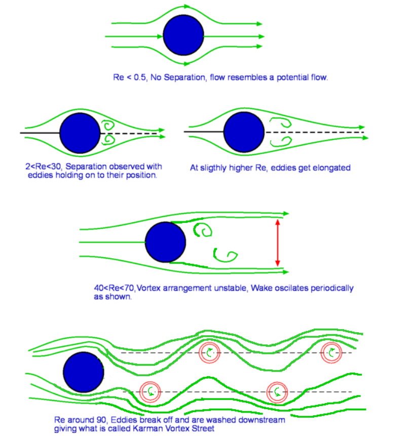 Figure 9 : Flow past a Circular Cylinder at various Reynolds Numbers 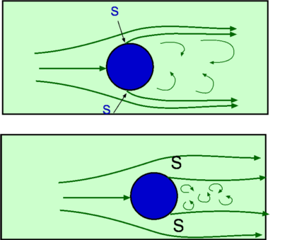 Figure 10 : Flow past a Circular Cylinder at various Reynolds Numbers, continued. In the Reynolds number range 104 to 105 A laminar boundary layer exists up to the vertical centreline of the cylinder (Fig.10). The flow separates at around this point S, which makes an angle of about 800 with the centre of the cylinder. A wide wake is seen downstream. The pressure in the separated region is almost constant. The observed CP distribution is shown in Fig 31 in the section on Potential Flow. The net pressure difference PA - PB contributes to pressure drag. A dramatic change takes place when the Reynolds number is around 2x10⁵ when the boundary layer becomes turbulent before separation. Now the separation is postponed since a turbulent boundary layer is able to sustain for a longer time than a laminar flow. The point of separation S now is found at 1300 as shown in Fig.10. The wake has now narrowed. The CP distribution indicates that the pressure in the wake is now higher than that for the laminar case (Fig. 31 Potential Flow Section). The consequence is that CD is now reduced to about 0.3. This reduction in drag around the cylinder is exploited in golf. The purpose of providing dimples on golf ball is to trip turbulence in order to decrease drag. Bowlers in cricket, especially those who bowl "swings" would like to have one side of the ball more smooth than the other. The idea is to keep flow on one side of the ball laminar and the other one turbulent. The ball will swing from the laminar to the turbulent side. Decrease in pressure drag can be achieved by delaying or stopping separation of flow. One of the strategies developed is to streamline the body. An aerofoil surface is an excellent example. In nature, bird wings and fish are examples of reduced drag bodies. Fig. 11 gives the numerical values of CD for some of the familiar two-dimensional shapes. It is clear that CD depends upon the orientation of the object to the flow. CD values for some of the three-dimensional objects are given in Fig. 12. 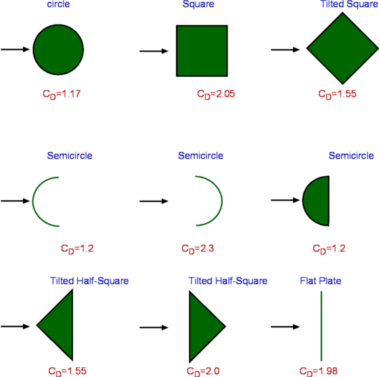 Figure 11 : CDvalues for familiar two-dimensional objects. 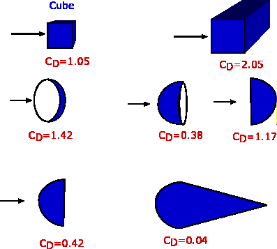 Figure 12 : CD Values for familiar three-dimensional objects |