Gas Dynamics &
|
Flow through Nozzles and Ducts
A subsonic flow responds to area changes in a similar manner as an incompressible flow. A supersonic flow behaves in an opposite manner in that when there is an area decrease, Mach Number decreases, while for an area increase, Mach Number increases. It this supersonic case a sonic flow can occur only at a throat, a section where area is the minimum. With this theory it is possible to explore the properties of gas flow through nozzles. Flow through a Converging NozzleThe first application of this theory is a converging nozzle connected to a reservoir where stagnation conditions prevail, $P = P_0, T = T_0 , u = 0$. By definition reservoirs are such that no matter how much the fluid flows out of them, the conditions in them do not change. In the reservoir it is assumed that pressure, temperature, density etc. remain the same always. The pressure level $P_b$ at the exit of the nozzle is referred to as the Back Pressure and it is this pressure that determines the flow in the nozzle. When the Back Pressure, $P_b$ is equal to the reservoir pressure, $P_r = P_0$ there is no flow in the nozzle. This is condition (1) in Fig. 18. If $P_b$ is reduced slightly to $P_2$ (condition (2)), a flow is induced in the nozzle. For relatively high values of $P_b$ , the flow is subsonic throughout. A further reduction in Back Pressure still results in a subsonic flow, but with a higher Mach Number at the exit (condition (3)). As $P_b$ is reduced we have an increased Mach Number at the exit along with an increased mass flow rate. This situation continues until a Back Pressure value is reached where the flow reaches sonic conditions ( $>M=1$ ) at the exit (4). This value of Back pressure follows from the isentropic equations. For air it is given by $$P_b^{\text"*"}/P_0=0.5283$$ When the Back Pressure is further reduced (5,6 etc.), the Mach Number at the exit tries to increase. It demands an increased mass flow from the reservoir. But as the condition at the exit is sonic, signals do not propagate upstream. The Reservoir is unaware of the conditions downstream and it does not send any more mass flow. Consequently the flow pattern remains unchanged in the nozzle. Any adjustment to the Back Pressure takes place outside of the nozzle. The nozzle is now said to be choked. The mass flow rate through the nozzle has reached its maximum possible value, the choked value. From the Fig. 18 it can be seen that there is an increase in mass flow rate only till choking condition (4) is reached. Thereafter mass flow rate remains constant. 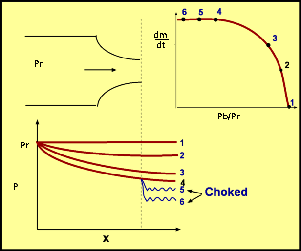 Figure 18 : Flow through a Converging Nozzle Note that for a non-choked flow, the Back Pressure and the pressure of the flow at the exit plane are equal. But when the nozzle is choked the two are different. The flow will need to adjust out side the exit of the nozzle. Usually this take place by means of expansion waves which reduce the exit pressure until it eventually equals the back pressure at a point down stream. Flow through a Converging-diverging nozzleA converging-diverging nozzle is called a de Laval nozzle, it is an essential element of a supersonic wind tunnel. In this application, the nozzle draws air from a reservoir with a fixed stagnation pressure. It is assumed that the back pressure at the end of the diverging section is such that air reaches sonic conditions at throat. The flow Mach Number increases in the diverging section. The area ratio and the back pressure can be set so that a required Mach Number is obtained at the end of the diverging section. Different area ratios give different Mach Numbers. The effect of Back Pressure on the flow through a converging-diverging nozzle is somewhat more complicated than that for a converging nozzle. Flow configurations for various back pressures and the corresponding pressure and Mach Number distributions are given in Fig. 19.
 Figure 19 : Pressure and Mach Number Distribution for the Flow through a Converging-Diverging Nozzle. Supersonic Nozzle ExperimentA typical method of familiarising students with the behaviour of supersonic gas flow is via the use of a supersonic nozzle experiment. The following section outlines a procedure for carrying out experiments to measure pressure ratio in a nozzle and observe flow patterns. 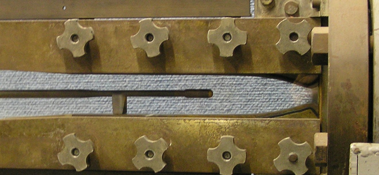 Figure 20 : 2-D Supersonic Flow Nozzle Experimental Equipment.The set up of the apparatus is shown in Figs 20, 21 and 22. The function of each piece of equipment is noted. A high-pressure gas supply line is attached to a reservior. The reservior is joined to the inlet of a converging-diverging nozzle. Flow is controlled via a manually operated valve on the supply line to the reservior. In this case Back Pressure, $P_b$, is constant and equal to the surrounding atmosphere pressure. Flow is created by increasing the pressure in the reservoir, $P_0$. Once the valve is open to give sufficient upstream stagnation pressure, the nozzle will choke giving Mach 1 flow at the throat. Downstream of the throat (area $A^\text"*"$) the flow Mach number will depend primarily on the area ratio of the channel ($A\/A^\text"*"$) and a supersonic flow slightly above Mach 2 will be obtained. 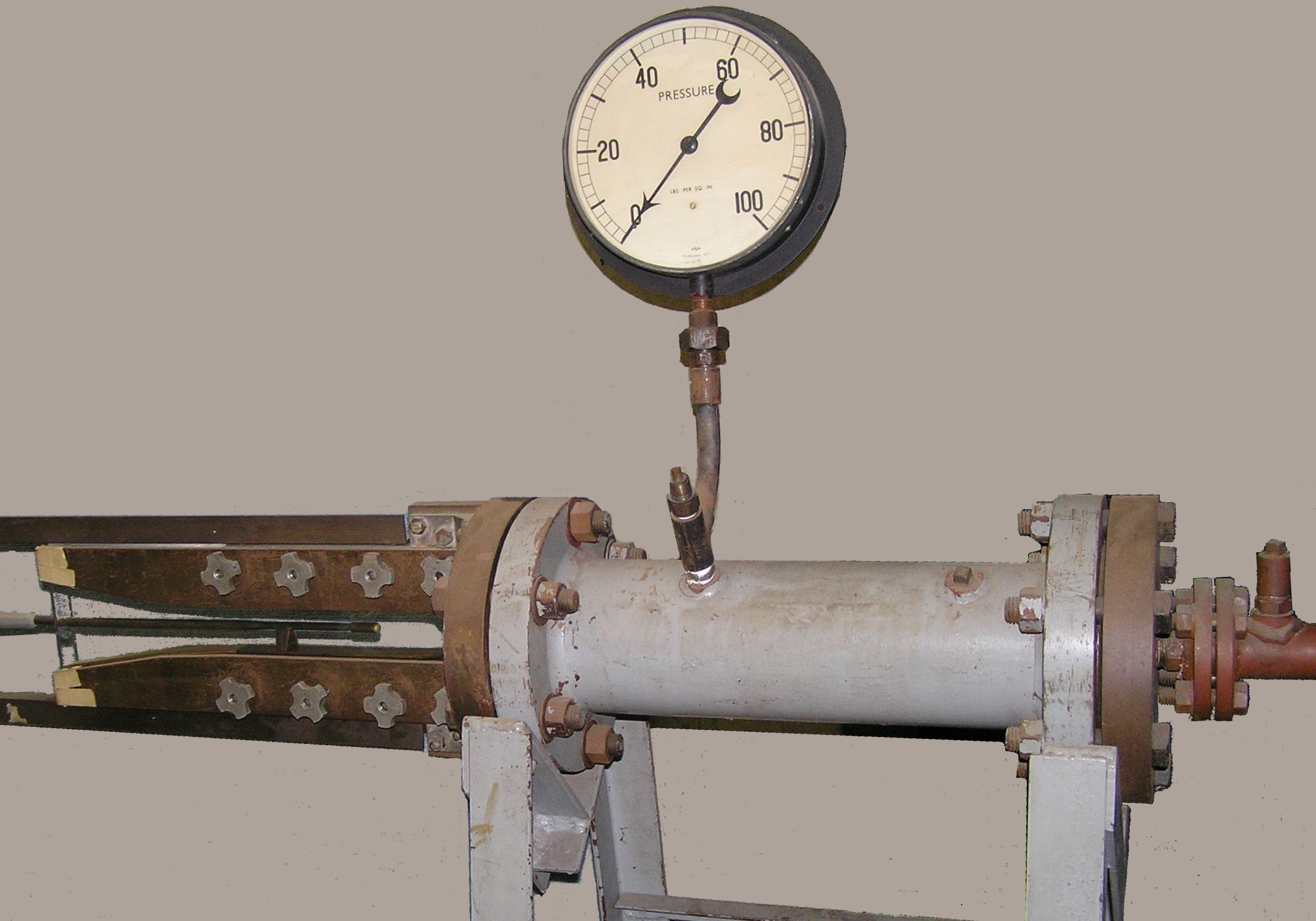 Figure 21 : High Pressure Supply System. A steel wall containing static pressure ports can be attached to the side of the nozzle. Using these ports, static pressure variation along the nozzle length can be determined. The static pressure to stagnation pressure ratio at any point along the channel can be used to predict local Mach number. This result can be compared to area ratio predictions and discrepancies due to boundary layer effects, shock waves or surface imperfections can be evaluated. A pitot pressure probe can be inserted into the flow at any station and can be used to predict upstream Mach number based on the stagnation pressure ratio change at that station. 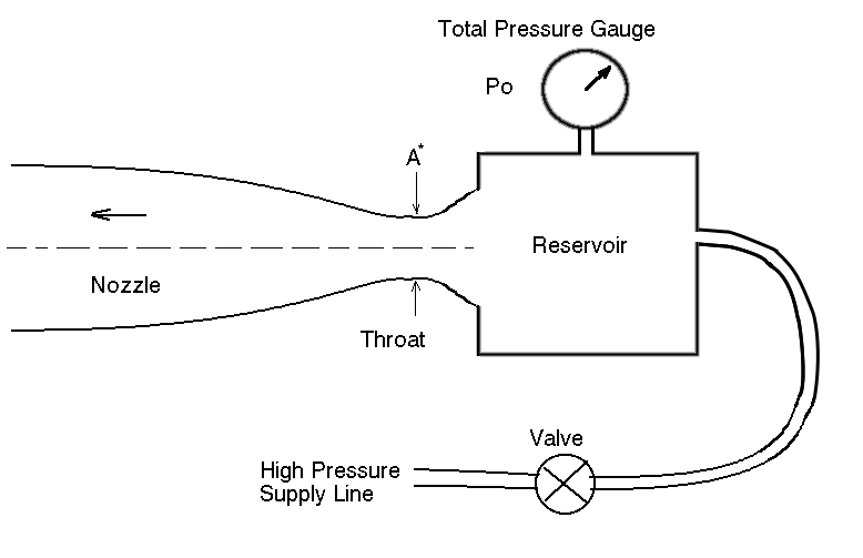 Figure 22 : Schematic of Equipment Connections. Nozzle GeometryNozzle static pressure port stations are shown in the following table. They are measured as distances downstream from the throat.
Throat Height ($A^\text"*"$) = 14.5 mm. Nozzle is two-dimensional with a constant depth, 25.4 mm Pressure measurementPressure measurement can be carried out using Piezo-electric transducers or conventional manometers. In this example mercury manometers are used to measure the pressures in the nozzle or upstream reservoir. 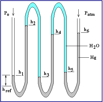 Stagnation pressure, $P_0$ is measured as the static pressure of the upstream reservoir where flow velocity is minimal. Since the stagnation pressure in this reservoir is quite high, a multi-column manometer has been used, rather than one very long single column. The mercury columns are joined by incompressible water columns. The final measure of stagnation pressure can be determined by addition of the mercury column heights and then subtracting the effect of the weight of water. $$P_0=(h_2-h_1)+(h_4-h_3)+(h_6-h_5)-{ρ_{H_2O}}/ρ_{Hg}((h2-h3)+(h_4-h_5))+Patm\text" cmHg "$$  Static pressure along the nozzle is obtained using a multitube manometer. Individual ports are connected in sequence. The axial position of the static pressure measurement points is shown in the previous table The first static port is located at station 1 which is downstream of the throat of the nozzle (station 0). Since the pressures drop below atmospheric then the values should be read from the manometer as follows. $$P=P_{atm}-h_i\text" cmHg "$$ Optical Measurement of Shock and Expansion Waves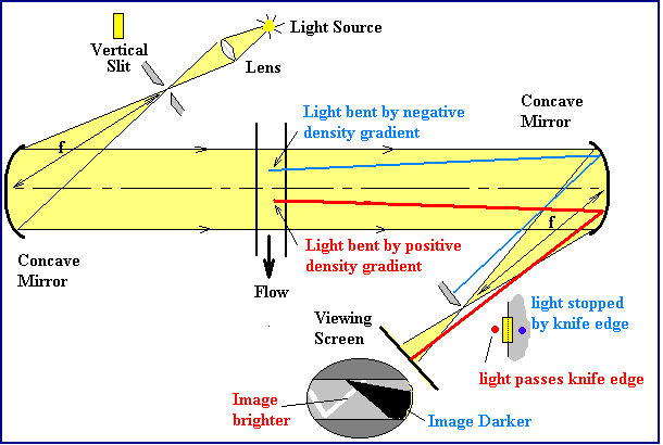 A Schleiren optical system can be used to visualise flow in the nozzle. This system uses the deflection of parallel light rays by the flow density gradients to produce visual images of the shock and expansion waves. A point light source shines on a concave mirror with a focal length such that a parallel beam of light is produced to illuminate the nozzle. Light rays passing through areas of high or low density gradient in the nozzle will be bent away from parallel. A matching pair concave mirror catches the light once it has gone through the nozzle and refocuses it onto a knife edge. The knife edge is set to allow about ½ of the light beam through to a viewing screen or camera. Light bent by expansions will be stopped at the knife edge. This missing light will cause dark areas on the screen where expansion waves occur. Light bent by compressions (shocks) will completely pass the knife edge and hence brighten these areas on the screen. The system can thus be used to produce images of supersonic flow. Some examples can be found here in the supersonic flow images page. Supersonic Nozzle SimulationNote: If you do not have access to a supersonic nozzle, a high pressure gas line or any of the other equipment mentioned above, then you can use the Supersonic Nozzle Simulation Software to carry out your experimental investigations. Experimental ProcedureTo carry out the experiments, follow the procedure outlined in the steps below.
Experimental Results
Data RecordingUse the following layout for recording manometer data for each nozzle run. Static Pressure Recordings. Static Pressure ports are located every 1/2 inch along the nozzle, starting with port 1 just downstream of the throat. Record Absolute Ambient Lab Pressure
The Stagnation Pressure of the flow is recorded in the reservoir upstream of the nozzle. Record Stagnation Pressure Data in the following table.
| |||||||||||||||||||||||||||||||||||||||||||||||||||||||||||||||||||||||||||||||||||||||||||||||||||||||||||||||||||||||||||||||||||||||