Gas Dynamics &
Supersonic Flow

Method of Characteristics

Numerical Example : Method of Characteristics Supersonic Nozzle Design

The Method of Characteristics is a very convenient tool to calculate isentropic portions within a supersonic flows. This is a numerical method, but the merit is that the method itself determines the grid (or mesh) it requires. Other CFD methods can be used for the same purpose but these require more extensive numerical calculations.

The mathematical theory behind the Method of Characteristics is based on the isentropic flow equations shown in previous sections, in particular the Prandtl-Meyer function.

Theory of Method of Characteristics

Governing Equations for a two-dimensional compressible, irrotational flow can be written as

The above equation is a statement that the flow is irrotational. These governing equations form a non-linear set of Partial Differential Equations. The solutions can be classified as follows,

• Elliptic, if $(u^2+v^2)\/a^2 < 1$
• Parabolic, if $(u^2+v^2)\/a^2 = 1$
• Hyperbolic, if $(u^2+v^2)\/a^2 > 1$.

Supersonic flows with $M > 1$, belong to the Hyperbolic class. One of the properties of Hyperbolic Equations is that there exist what are called the characteristic lines or directions. In a supersonic flow at every point there can exists small disturbance waves called Mach Waves. These are, in fact, the characteristic lines. The Direction of Mach Waves is the characteristic direction. Across a characteristic line, velocity derivatives may be discontinuous, but velocity itself will be discontinuous. Along the characteristic lines, the Compatibility Relations hold good.

Compatibility Relations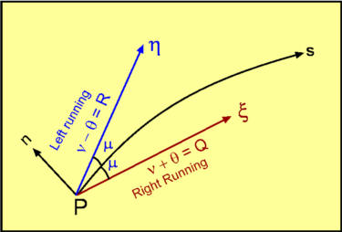

Figure 51: Riemann Invariants

A stream line in a supersonic flow as in Fig. 51. The coordinate $s$ axis is aligned along the streamline and the other axis $n$, normal to it. The are two Mach lines at a point $(P)$. The one to the left of the streamline is a $η$ characteristic and the one to the right is called an $ξ$ characteristic. Note that each of these is inclined at an angle $μ$ to the streamline. It can be shown that along an $η$ characteristic,

i.e.,

Similarly along a $ξ$ characteristic,

i.e,

The above equations are the Compatibility Relations. Essentially, they say that $Q$ and $R$ are invariant in $ξ$ and $η$ directions respectively. These are known as Riemann Invariants and are relatively simple because of the application they are being applied to here.

Computing with Method of Characteristics

Working with the Method of Characteristics is relatively easy if the problem is formulated in terms of $ν$ and $θ$. Once these two variables are determined at any point in the flow, other quantities of interest such as Mach Number, flow velocity and pressure can be determined using isentropic relations. Accordingly, consider a curve AB in the flow along which $ν$ and $θ$ are known. This curve is known as a Starting Curve. The procedure to calculate values at point (C) are shown in Fig. 52.

Now,

Solving for $ν_C$ and $θ_C$ , gives

or in more general terms,

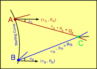Figure 52 : Computing using Method of Characteristics

Once the flow at (C) is calculated, it is possible to continue and calculate the flow downstream.

In practice, to gain accuracy, a number of points on the starting curve are considered. Mach Lines are drawn from each of them. Then the procedure marchs downstream calculating the flow at every subsequent point. In this process, a net or a grid of points is created as shown in Fig. 53.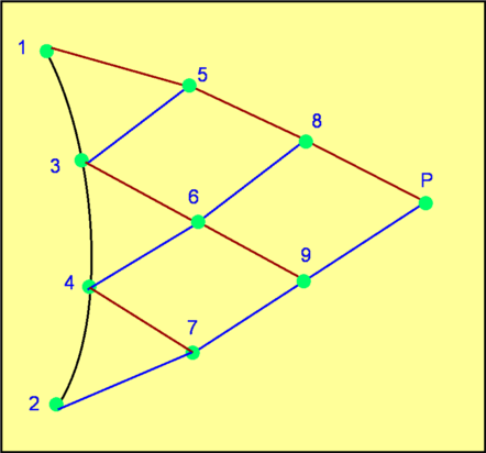

Figure 53: The Method of Characteristics Procedure

Note that the characteristics are approximated by straight lines. For example consider Fig. 54. The characteristic at (4)or (2) is treated as a straight line. This is true only if Mach Number is constant between (4) and (7) or between (2) and (7). If the Mach Number varies between these points then the true solution are curves which intersect at (7') instead of (7). Therefore what is calculated as properties for point (7) are actually those at point (7'). The error due to this approximation may be minimised by bringing (2) and (4) closer. In other words a large number of points on the Starting Curve makes the solution more accurate.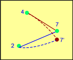

Figure 54 : Accuracy of the Procedure

The procedure needs to be modified near a solid boundary or a free boundary. At a solid boundary the flow inclination is fixed i.e., $θ = \text"Constant"$. At a free boundary $ν = \text"Constant"$. These effects can be seen in the example given below.

Flow through a Diverging Duct

Consider a flow at Mach 1.605 entering a two-dimensional diverging duct whose sides make an angle of 6^o with the centreline, ie., a 12^o divergence. It is required to calculate the flow in the duct. See Fig. 55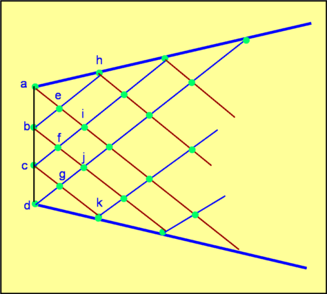

Figure 55 : Flow through a Diverging Duct

Four points are selected on the starting line - (a), (b), (c) and (d). At each of these points Mach Number is the same, 1.605 or $ν=15^o$. The flow will be horizontal on the centreline and will be aligned with the wall at the two side boundaries. Accordingly, $θ$ will be 6^o,2^o,-2^o and -6^o at (a), (b), (c) and d respectively. The staring values are tabulate below.

Interior Point

Consider Point (e), then,

From this value of $ν$, this infers a Mach Number of 1.672.

Boundary Point

Consider the boundary point (h),

Mach Number corresponding to $ν=19^o$ is 1.741.

This proceedure can be continued at the remaining points in the flow. Note: the grid is not fixed but constructed as the procedure is marched throught the flow field. Angles for the characteristic lines are determined by the value of $μ$ and $θ$ at each upstream point.

Cancellation of Waves

In many applications the cancelation of waves may be required. This happens in situations such as a supersonic nozzle where a test section with uniform flow free of all waves and further expansion is required. The principle behind the cancellation follows directly from the methods shown above.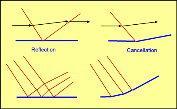

Figure 56 : Reflection and cancellation of Waves

Consider the wave reflection from a wall as shown in Fig. 56. By suitably turning the wall to equal the $θ$ value of the characteristic, the wave can be cancelled and the downstream value of $ν$ will remain unchanged. This also applies to a series of waves.

Design of a Supersonic Nozzle

A supersonic nozzle is the basic element of any supersonic wind tunnel and its geometry is what accelerates the flow to the required Mach Number $M_T$ at the test section. A converging-diverging nozzle as shown in Fig. 57. The converging section of the nozzle is provided to obtain sonic conditions at the throat. The geometry of this section is somewhat arbitrary as it is purely accelerating subsonic flow. But should not be too abrupt as to cause flow separation at the throat.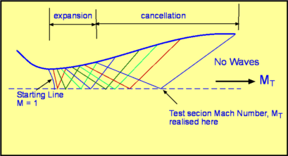

Figure 57 :Design of a Supersonic Nozzle, only upper half shown

The critical component of a supersonic nozzle is the design of the diverging section. The conditions at the throat are sonic, i.e., $ν=0$, while at the exit section there is a Mach Number, $M_T$ or a value of $ν = ν_T$. It is required that the flow be turned through an angle equal to $ν_T$. In theory it is possible to effect this in one "go", ie. turning the flow through $ν_T$ at a sharp corner. But in reality this is not an efficient design. A sudden turn could result in separation of flow. Further, it is required that the flow entering the test section be uniform, implying the absence of any expansion waves downstream. A Method of Characteristics procedure will produce a near optimal design.

The flow expansion in the diverging section is carried out in two stages - (a) Expansion Section and (b) Straightening Section. In the Expansion Section flow is expanded up to $θ_{max}$ . In the subsequent Straightening Section, $θ$ is reduced progressively to cancel the waves. When complete $θ = 0$ on the walls and $ν = ν_T$ at the centreline. Each of these operations can be carried out in a number of steps as per the above Method of Characterists procedures. Fig. 57 shows the general process.

The value of $θ_{max}$ will depend on the required exit Mach number, $M_T$, and the desired length of the nozzle. By iteration it is possible to minimise this length. In many cases, the the Expansion Section can be kept at zero length. It will have a Prandtl-Meyer expansion at the throat as shown in Fig. 58.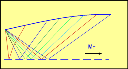

Figure 58: Design of a Minimum Length Supersonic Nozzle, only upper half shown

See Method of Characteristics Nozzle Design script for an example impletation of this theory.